16.38. jitter_solve
The jitter_solve program takes as input several overlapping images and
linescan and/or frame camera models in CSM format (such as for LRO NAC, CTX,
HiRISE, Airbus Pleiades, DigitalGlobe, etc., Section 8.12) and adjusts each
individual camera position and orientation in the linescan model to make them
more consistent with each other and to the ground.
The goal is to reduce the effect of unmeasured perturbations in the
linescan sensor as it acquires the data. This is quite analogous to
what bundle_adjust does (Section 16.5), except that the
latter tool has just a single position and orientation per camera,
instead of a sequence of them.
Usage:
jitter_solve <images> <cameras> <input adjustments> \
  -o <output prefix> [options]
16.38.1. Limitations
When the scan lines from the images are nearly parallel to each other the jitter cannot be fully disambiguated, and some residual jitter is left unsolved.
Best results are achieved if scan lines from one image cross blocks of scan lines from another image that correspond to at least one jitter period. In practice, for WorldView images, for example, the across-track angle can vary notably from one image to another, resulting in such a favorable regime.
If the prior DEM used as constraint (Section 16.38.2.2) has
systematic differences with what is expected from the images, this can bias the
results. Potential solutions are to mask the problematic areas in the DEM and /
or use a value of --heights-from-dem-uncertainty that is quite a lot larger
than the actual uncertainty.
GCP files produced from a prior DEM of good quality can help increase the accuracy (Section 16.18).
A larger number of images (more than two, ideally with scan lines notably crossing each other) can improve the results.
It is strongly recommended to use this solver with carefully set camera position constraints and with anchor points, to prevent oscillations in the solution (Section 16.38.2). An example is in Section 11.10.22.
More research is needed about how to set up parameters for this solver in various situations.
If frame camera images exist for the same extent, they will help solve for jitter, as such images are rigid across scan lines.
16.38.2. Ground constraints
Optimizing the cameras to reduce the jitter and make them self-consistent can result in the camera system moving away from the initial location or warping of any eventually produced DEM.
Hence, ground and camera constraints are very important. In fact, it is strongly
recommended to always use both the camera position uncertainty
(--camera-position-uncertainty, Section 16.38.3) and anchor points
(--num-anchor-points or --num-anchor-points-per-tile, together
with --anchor-dem and --anchor-dem-uncertainty,
Section 16.38.6). These two together constrain the camera position
and orientation, respectively. Without them the problem can be under-constrained
and the solution can become unstable, especially for linescan cameras and where
there are no interest point matches (such as over clouds and shadows).
All the ground constraints in this tool are specified as an uncertainty
(1-sigma) in meters, so they can be reasoned about and balanced against each
other: the GCP sigma (Section 16.5.9), --heights-from-dem-uncertainty,
--anchor-dem-uncertainty. Then, there is the triangulation constraint
(--tri-weight, internally divided by the GSD, so this is dimensionless).
This tool uses several kinds of constraints. They are described below, and an example of comparing different ground constraints is given in Section 16.38.10.
16.38.2.1. Triangulated point constraint
Triangulated ground points obtained from interest point matches are kept, during optimization, close to their initial values. This works well when the images have very good overlap.
This is controlled by the option --tri-weight whose default value is 0.1.
This is divided by the image GSD when computing the cost function, to make the
distances on the ground in units of pixels.
A report file having the change in triangulated points is written to disk (Section 16.38.17.3). It can help evaluate the effect of this constraint. Also check the pixel reprojection errors per camera (Section 16.38.17.2) and per triangulated point (Section 16.38.17.6), before and after solving for jitter.
Triangulated points that are constrained via a DEM (option
--heights-from-dem, Section 16.38.2.2), that is, those that
are near a valid portion of this DEM, are not affected by the triangulation
constraint.
The implementation is just as for bundle adjustment (Section 16.5.6.1).
An example is given in Section 16.38.9. See Section 16.38.18 for the full description of this option.
16.38.2.2. Reference DEM constraint
This ties the triangulated ground points obtained from interest point matches to an external DEM, which may be at a lower resolution than the images. It is expected that this external DEM is well-aligned with the input cameras (see Section 16.53.14 for how to do the alignment).
This option is named --heights-from-dem, and it is controlled via
--heights-from-dem-uncertainty and --heights-from-dem-robust-threshold.
The use of these options is shown in Section 16.38.8.
The previously mentioned triangulated point constraint will be employed where the triangulated points are not close to the DEM given by this option.
The DEM constraint is preferred, if a decent DEM that is well-aligned with the cameras is available.
If the difference between the stereo DEM before jitter correction and the
reference DEM is large, the value of --heights-from-dem-uncertainty should
be increased. If the reference DEM has systematic differences, such as due to
vegetation, this constraint may need to be omitted, or have the systematic
differences masked.
An example with and without this constraint is shown in Section 16.38.10.
See also Section 16.38.1 for limitations of this constraint.
The implementation of this constraint is the same as for bundle adjustment (Section 12.2.1.3).
This solver can also use a sparse point cloud as a constraint. This is an advanced option. See Section 16.38.16.
16.38.2.3. Ground control points
Just like bundle_adjust (Section 16.5.9), this program can make use of
ground control points. The pixel residuals at ground control points
are flagged in the produced report file (Section 16.38.17.6).
Ground control points can be produced by tying a stereo DEM to a different high quality DEM (Section 16.18).
16.38.3. Camera constraints
Jitter is believed to be caused by vibrations in the linescan camera as it acquires the image. If that is the case, the camera positions are likely accurate, and can be constrained to not move much, while the orientations can move more.
If estimates for the horizontal and vertical camera position uncertainties
exist, per camera, these can be incorporated into the optimization via the option
--camera-position-uncertainty. It is good to use those uncertainties
generously, so to set them to be larger than the actual uncertainty.
See the bundle_adjust documentation at Section 16.5.6.2
for an example and implementation details.
This program writes report files that record the changes in camera position (Section 16.38.17.3) and the resulting pixel reprojection errors per camera (Section 16.38.17.2).
It is suggested to examine these and adjust the camera constraints, if needed. A tight constraint can prevent convergence and result in large reprojection errors.
An alternative constraint, --camera-position-weight, can be set to a large
value, on the order of 1e+4, to effectively keep the camera positions in place.
This is an older option that will be removed.
Camera position and ground constraints should be sufficient. It is suggested not
to use the experimental --rotation-weight option.
16.38.3.1. Smoothness constraint
The option --smoothness-weight constrains how much each sequence of
linescan poses can change in curvature relative to the initial values.
This can prevent convergence.
A range of values is suggested in Section 16.38.18.
16.38.3.2. Roll and yaw constraints
Other related options that may improve the regularity of the camera poses
are --roll-weight and --yaw-weight (they should be used with the
--initial-camera-constraint option).
It is strongly suggested not to use these (or the smoothness weight) in a first pass. Only if happy enough with the results and it is desired to control various aspects of the solution, one should try these options.
Values for these are suggested in Section 16.38.18.
16.38.4. Resampling the poses
Oftentimes, the number of tabulated camera positions and orientations in the CSM file is very small. For example, for Airbus Pleiades, the position is sampled every 30 seconds, while acquiring the whole image can take only 1.6 seconds. For CTX the opposite problem happens, the orientations are sampled too finely, resulting in too many variables to optimize.
Hence, it is strongly suggested to resample the provided positions and
orientations before the solver optimizes them. Use the options:
--num-lines-per-position and --num-lines-per-orientation. The
estimated number of lines per position and orientation will be printed
on screen, before and after resampling.
In the two examples below drastically different sampling rates will be used. Inspection of residual files (Section 16.38.17), and of triangulation errors (Section 14.6.1) and DEM differences after solving for jitter (Section 16.38.9) can help decide the sampling rate.
16.38.5. Interest point matches
Solving for jitter is a fine-grained operation, modifying many positions
and orientations along the satellite track. Hence, many dense and
well-distributed interest points are necessary. It is suggested to create these
with pairwise stereo, with the option --num-matches-from-disparity
(Section 12.2.4.2). An example is shown in Section 16.38.8. An alternative
to pairwise stereo is discussed below.
The most accurate interest points are obtained when the images are mapprojected. This is illustrated in Section 16.38.9. The produced interest point matches will be, however, between the original, unprojected images, as expected by the solver.
It was found experimentally that the best dense interest point matches are
obtained by invoking parallel_stereo with the options --stereo-algorithm
asp_bm and --subpixel-mode 1. The asp_mgm algorithm
(Section 6.1.1), while producing more pleasing results, smears
somewhat the interest points which makes solving for subpixel-level accurate
jitter less accurate.
Pass these disparity-based matches to the jitter solver with
--match-files-prefix, using their run-disp prefix. Renaming them is
error-prone when the image names are long, as that can invalidate the shortening
of long match file names (Section 19.11).
If having more than two images, one can do pairwise stereo to get dense matches. For a large number of images this is prohibitive.
Sparse interest point matches can work almost as well if sufficiently
well-distributed and accurate. Then stereo is not necessary. Use
parallel_bundle_adjust with the options --ip-detect-method 1 to create
subpixel-level accurate matches, and with --ip-per-tile 500 --matches-per-tile
500 to ensure there are plenty of them. The option --mapprojected-data
(Section 12.2.4.3) is suggested as well.
It is suggested to call jitter_solve with a large value of
--max-pairwise-matches, such as 40000, or 2-3 times more than that for
images with lots of lines and high-frequency jitter. There must be at least
a handful of matches for each jitter period.
Examine the interest point matches in stereo_gui
(Section 16.72.9). Also examine the produced pointmap.csv files
to see the distribution and residuals of interest points
(Section 16.38.17.6), and if the matches are dense enough given the
observed jitter.
This program can read interest point matches in the ISIS control network format,
using the option --isis-cnet, and from an NVM file, with the option
--nvm.
See Section 16.5.10 in the bundle_adjust manual for more details
about control networks. Unlike that program, jitter_solve does not save an
updated control network, as this tool changes the triangulated points only in
very minor ways. Camera poses from NVM files are not read either.
16.38.6. Anchor points
The anchor points are created based on pixels that are uniformly distributed over each image, not just where the images overlap, and can even go beyond the first and last image line. This ensures that the optimized poses do not oscillate where the images overlap very little or not at all, such as over clouds and shadows, where there may be no interest point matches.
This constraint works by projecting rays to the ground from the chosen uniformly distributed pixels, finding the anchor points where the rays intersect the anchor DEM, then adding to the cost function the reprojection errors (Section 12) for the anchor points. This complements the reprojection errors from triangulated interest point matches, and the external DEM constraint (if used).
The purpose of the anchor points is to control the camera orientation, by
constraining how much the ground points, where the rays meet the anchor DEM, are
allowed to move. The strength of this constraint is set with
--anchor-dem-uncertainty, the uncertainty of the anchor points, as a 1-sigma
value in meters. A smaller value constrains the cameras more. This option was
introduced in build 2026/6 (Section 2.1).
This constraint is normally used together with the camera position uncertainty
(--camera-position-uncertainty, Section 16.38.3). These two together
fully constrain the problem: the camera position uncertainty controls where the
cameras are, while the anchor points control the orientation by holding the
ground points in place. It is important to normally set both, as otherwise the
problem is under-constrained, especially when there are no interest point matches
in certain areas, such as over clouds and shadows.
The anchor uncertainty should normally be notably larger than
--heights-from-dem-uncertainty (Section 16.38.2.2). Otherwise
the anchor constraint is too strong and convergence may be prevented.
Specifying the uncertainty in meters is preferred to the older --anchor-weight
option, which is harder to interpret. This way the ground constraints that are
expressed as uncertainties (ground control points, the DEM constraint, and the
anchor points constraint) are in the same units of meters, which makes them
easier to reason about and to balance against each other. (The triangulation
constraint, --tri-weight, is the exception, being a weight, not an
uncertainty.) The two options are mutually exclusive; an anchor weight w
corresponds to an anchor DEM uncertainty of 1/w.
Anchor points are strongly encouraged either with a triangulated point constraint
or a reference DEM constraint. To avoid the anchor points dominating the problem,
their number should be less than the number of interest point matches (and of the
triangulated and DEM-constrained points), and their uncertainty
(--anchor-dem-uncertainty) should be larger than
--heights-from-dem-uncertainty. Resampling the camera poses very finely may
require more anchor points.
The solver prints to the terminal the total number of triangulated points, anchor points, and ground control points. This helps check that these counts are balanced.
A report file that has the residuals at anchor points is written down (Section 16.38.17.7). The per-image counts and total number of anchor points are printed on the terminal.
The relevant options are --num-anchor-points,
--num-anchor-points-per-tile, --anchor-dem-uncertainty, --anchor-dem,
and --num-anchor-points-extra-lines. An example is given in
Section 16.38.9.
16.38.7. Solving for intrinsics
For some datasets there can be both jitter and lens distortion effects, such as for Kaguya TC (Section 12.2.2, Section 8.14.8). In such cases, the stronger phenomenon should be solved for first.
The bundle_adjust and jitter_solve programs can use each other’s output
cameras as inputs, as each saves image and optimized camera lists
(Section 16.5.11.7), which can then be passed in to the other program
via the --image-list and --camera-list options.
16.38.8. Example 1: CTX images on Mars
A CTX stereo pair will be used which has quite noticeable jitter. See Section 16.38.8.5 for a discussion of multiple images, and a similar example for KaguyaTC in Section 8.14.8.
See also Section 16.38.1 for limitations of this constraint.
16.38.8.1. Input images
The pair consists of images with ids:
J03_045820_1915_XN_11N210W
K05_055472_1916_XN_11N210W
See Section 8.3 for how to prepare the image files and Section 8.12.2.1 for how to create CSM camera models.
All produced images and cameras were stored in a directory named
img.
16.38.8.2. Reference datasets
The MOLA dataset from:
is used for alignment. The data for the following (very generous)
longitude-latitude extent was fetched: 146E to 152E, and 7N to 15N. The obtained
CSV file was saved as mola.csv. See Section 19.12.4 for the
--csv-format to use, and Section 16.56.3 for the MOLA data flavors and
datums.
A gridded DEM produced from this unorganized set of points is shipped with the ISIS data. It is gridded at 463 meters per pixel, which is quite coarse compared to CTX images, which are at 6 m/pixel, but it is good enough to constrain the cameras when solving for jitter. A clip can be cut out of it with the command:
gdal_translate -co compress=lzw -co TILED=yes \
-co INTERLEAVE=BAND -co BLOCKXSIZE=256 -co BLOCKYSIZE=256 \
-projwin -2057237.6 1077503.1 -1546698.4 275566.33 \
$ISISDATA/base/dems/molaMarsPlanetaryRadius0005.cub \
ref_dem_shift.tif
This one has a 190 meter vertical shift relative to the preferred Mars radius of 3396190 meters, which can be removed as follows:
image_calc -c "var_0-190" -d float32 ref_dem_shift.tif \
-o ref_dem.tif
As a sanity check, one can take the absolute difference of this DEM and the MOLA csv file as:
geodiff --absolute --csv-format 1:lon,2:lat,5:radius_m \
mola.csv ref_dem.tif
This will give a median difference of 3 meters, which is about right, given the uncertainties in these datasets.
A DEM can also be created from MOLA data with point2dem
(Section 16.56):
point2dem -r mars --tr 500 \
--stereographic --auto-proj-center \
--csv-format 1:lon,2:lat,5:radius_m \
--search-radius-factor 10 \
mola.csv
This DEM can be blurred with dem_mosaic, with the option --dem-blur-sigma
5.
16.38.8.3. Uncorrected DEM creation
Bundle adjustment is run first:
bundle_adjust \
--ip-per-image 20000 \
--max-pairwise-matches 100000 \
--tri-weight 0.1 \
--tri-robust-threshold 0.1 \
--camera-weight 0 \
--remove-outliers-params '75.0 3.0 10 10' \
img/J03_045820_1915_XN_11N210W.cal.cub \
img/K05_055472_1916_XN_11N210W.cal.cub \
img/J03_045820_1915_XN_11N210W.cal.json \
img/K05_055472_1916_XN_11N210W.cal.json \
-o ba/run
The triangulation weight was used to help the cameras from drifting. Outlier removal was allowed to be more generous (hence the values of 10 pixels above) as perhaps due to jitter some triangulated points obtained from interest point matches may not project perfectly in the cameras.
Here we chose to use a large value for --max-pairwise-matches and
we will do the same when solving for jitter below. That is because
jitter-solving is a finer-grained operation than bundle adjustment,
and a lot of interest point matches are needed.
It is very important to inspect the final_residuals_stats.txt report file to
ensure each image has had enough features and has small enough reprojection
errors (Section 16.5.11).
Stereo is run next. The local_epipolar alignment (Section 6.1)
here did a flawless job, unlike affineepipolar alignment which resulted in
some blunders.
parallel_stereo \
--bundle-adjust-prefix ba/run \
--stereo-algorithm asp_mgm \
--num-matches-from-disparity 40000 \
--alignment-method local_epipolar \
img/J03_045820_1915_XN_11N210W.cal.cub \
img/K05_055472_1916_XN_11N210W.cal.cub \
img/J03_045820_1915_XN_11N210W.cal.json \
img/K05_055472_1916_XN_11N210W.cal.json \
stereo/run
point2dem --stereographic --auto-proj-center \
--errorimage stereo/run-PC.tif
Note how above we chose to create dense interest point matches from
disparity. They will be used to solve for jitter. We used the option
--num-matches-from-disparity. See Section 16.38.5 for
more details.
See Section 6 for a discussion about various speed-vs-quality choices for stereo. Consider using mapprojected images (Section 6.1.7).
We chose to use here a local stereographic projection (Section 16.56.1).
This DEM was aligned to MOLA and recreated, as:
pc_align --max-displacement 400 \
--csv-format 1:lon,2:lat,5:radius_m \
stereo/run-DEM.tif mola.csv \
--save-inv-transformed-reference-points \
-o stereo/run-align
point2dem --stereographic --auto-proj-center \
stereo/run-align-trans_reference.tif
The value in --max-displacement may need tuning
(Section 16.53).
This transform was applied to the cameras (note that this approach is applicable only
when the first cloud in pc_align was the ASP-produced DEM, otherwise see Section 16.53.14):
bundle_adjust \
--input-adjustments-prefix ba/run \
--initial-transform stereo/run-align-inverse-transform.txt \
img/J03_045820_1915_XN_11N210W.cal.cub \
img/K05_055472_1916_XN_11N210W.cal.cub \
img/J03_045820_1915_XN_11N210W.cal.json \
img/K05_055472_1916_XN_11N210W.cal.json \
--apply-initial-transform-only \
-o ba_align/run
16.38.8.4. Solving for jitter
Then, jitter was solved for, using the original cameras, with the adjustments prefix having the latest refinements and alignment:
jitter_solve \
img/J03_045820_1915_XN_11N210W.cal.cub \
img/K05_055472_1916_XN_11N210W.cal.cub \
img/J03_045820_1915_XN_11N210W.cal.json \
img/K05_055472_1916_XN_11N210W.cal.json \
--input-adjustments-prefix ba_align/run \
--max-pairwise-matches 100000 \
--match-files-prefix stereo/run-disp \
--num-lines-per-position 1000 \
--num-lines-per-orientation 1000 \
--max-initial-reprojection-error 20 \
--camera-position-uncertainty 2000,2000 \
--heights-from-dem ref_dem.tif \
--heights-from-dem-uncertainty 20.0 \
--num-iterations 50 \
--anchor-dem ref_dem.tif \
--num-anchor-points 1000 \
--anchor-dem-uncertainty 50.0 \
--tri-weight 0.1 \
-o jitter/run
It can be preferable to specify here the cameras after bundle adjustment, and
then omit --input-adjustments-prefix.
It was found that using about 1000 lines per pose (position and orientation) sample gave good results, and if using too few lines, the poses become noisy.
Either dense and uniformly distributed interest point matches or sufficiently dense subpixel-level accurate sparse matches are necessary to solve for jitter (Section 16.38.5).
Here anchor points were used. They can be necessary to stabilize the orientations (Section 16.38.6).
The constraint relative to the reference DEM is needed, to make sure the DEM produced later agrees with the reference one. Otherwise, the final solution may not be unique, as a long-wavelength perturbation consistently applied to all obtained camera trajectories may work just as well.
We used camera position constraints (Section 16.38.3), it is suggested to be generous with the uncertainties. For CTX they are likely rather large.
The report files mentioned in Section 16.38.17 can be very helpful in evaluating how well the jitter solver worked, even before rerunning stereo.
The model states (Section 8.12.6) of optimized cameras are saved with names like:
jitter/run-*.adjusted_state.json
Then, stereo can be redone, just at the triangulation stage, which is much faster than doing it from scratch. The optimized cameras were used:
parallel_stereo \
--prev-run-prefix stereo/run \
--stereo-algorithm asp_mgm \
--alignment-method local_epipolar \
img/J03_045820_1915_XN_11N210W.cal.cub \
img/K05_055472_1916_XN_11N210W.cal.cub \
jitter/run-J03_045820_1915_XN_11N210W.cal.adjusted_state.json \
jitter/run-K05_055472_1916_XN_11N210W.cal.adjusted_state.json \
stereo_jitter/run
point2dem --stereographic --auto-proj-center \
--errorimage stereo_jitter/run-PC.tif
To validate the results, first the triangulation (ray intersection) error (Section 16.56) was plotted, before and after solving for jitter. These were colorized as:
colormap --min 0 --max 10 stereo/run-IntersectionErr.tif
colormap --min 0 --max 10 stereo_jitter/run-IntersectionErr.tif
The result is below.
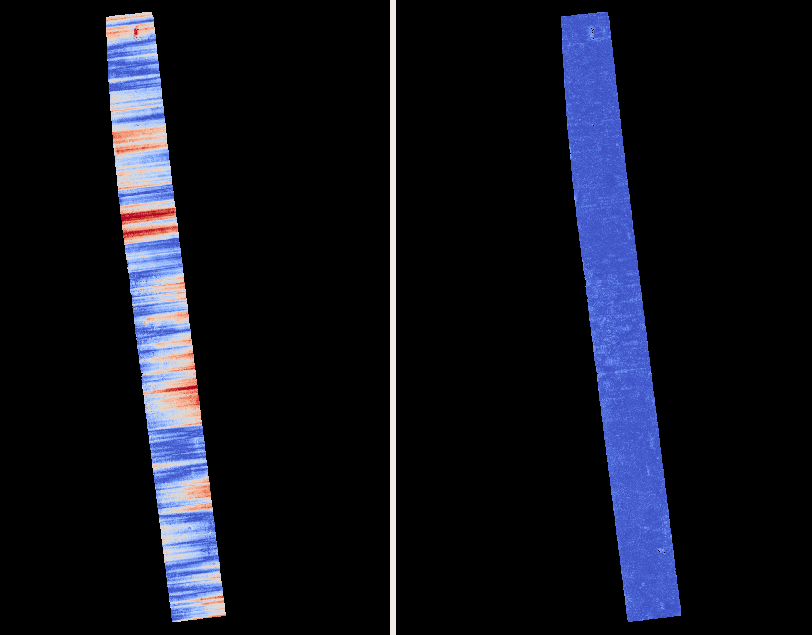
Fig. 16.7 The colorized triangulation error (max shade of red is 10 m) before and after optimization for jitter.
Then, the absolute difference was computed between the sparse MOLA dataset and the DEM after alignment and before solving for jitter, and the same was done with the DEM produced after solving for it:
geodiff --absolute \
--csv-format 1:lon,2:lat,5:radius_m \
stereo/run-align-trans_reference-DEM.tif mola.csv \
-o stereo/run
geodiff --absolute \
--csv-format 1:lon,2:lat,5:radius_m \
stereo_jitter/run-DEM.tif mola.csv \
-o stereo_jitter/run
Similar commands are used to find differences with the reference DEM:
geodiff --absolute ref_dem.tif \
stereo/run-align-trans_reference-DEM.tif -o \
stereo/run
colormap --min 0 --max 20 stereo/run-diff.tif
geodiff --absolute ref_dem.tif \
stereo_jitter/run-DEM.tif \
-o stereo_jitter/run
colormap --min 0 --max 20 stereo_jitter/run-diff.tif
Plot with:
stereo_gui --colorize --min 0 --max 20 \
stereo/run-diff.csv \
stereo_jitter/run-diff.csv \
stereo/run-diff_CMAP.tif \
stereo_jitter/run-diff_CMAP.tif \
stereo_jitter/run-DEM.tif \
ref_dem.tif
DEMs can later be hillshaded.
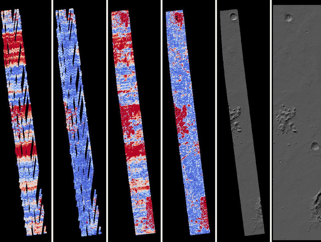
Fig. 16.8 From left to right are shown colorized absolute differences of (a) jitter-unoptimized but aligned DEM and ungridded MOLA (b) jitter-optimized DEM and ungridded MOLA (c) unoptimized DEM and gridded MOLA (d) jitter-optimized DEM and gridded MOLA. Then, (e) hillshaded optimized DEM (f) hillshaded gridded MOLA (which is the reference DEM). The max shade of red is 20 m difference.
It can be seen that the banded systematic error due to jitter is gone, both in the triangulation error maps and DEM differences. The produced DEM still disagrees somewhat with the reference, but we believe that this is due to the reference DEM being very coarse, per plots (e) and (f) in the figure.
16.38.8.5. Multiple CTX images
Jitter was solved jointly for a set of 27 CTX images with much overlap. The extent was roughly between -157.8 and -155.5 degrees of longitude, and from -0.3 to 3.8 degrees of latitude.
Bundle adjustment for the entire set was run as before. The
convergence_angles.txt report file (Section 16.5.11.4) was used to
find stereo pairs. Only stereo pairs with a median convergence angle of at least
5 degrees were processed, and which had at least several dozen shared interest
points. This resulted in 42 stereo pairs.
The resulting stereo DEMs can be mosaicked with dem_mosaic
(Section 16.20). Alignment to MOLA can be done as before, and the
alignment transform must be applied to the cameras (Section 16.53.14).
Then, jitter was solved for, as earlier, but for the entire set at once. Dense pairwise matches were used (Section 12.2.4.2). They were copied from individual stereo directories to a single directory. It is important to use the proper naming convention (Section 16.5.10.1). Care is needed when renaming the match files if the input image names are very long, as that can be error-prone (Section 19.11).
One could augment or substitute the dense matches with subpixel-level accurate sparse matches from bundle adjustment if renamed to the proper convention (Section 16.38.5). This can be helpful to ensure all images are tied together.
The DEM used as a constraint can be either the existing gridded MOLA product, or
it can be created from MOLA with point2dem (Section 16.38.8.2).
Here the second option was used. Consider adjusting the value of
--heights-from-dem-uncertainty. Tightening the DEM constraint is
usually not problematic, if the alignment to the DEM is good.
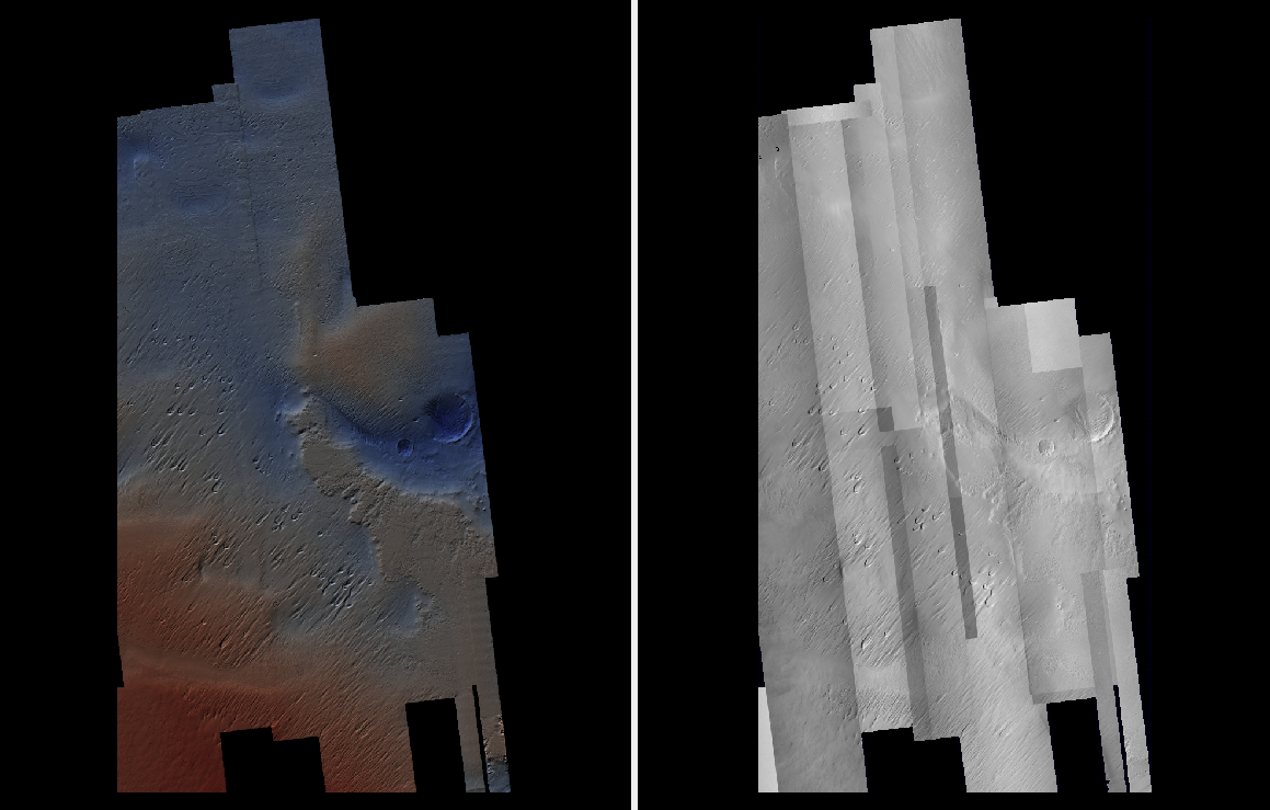
Fig. 16.9 DEM and orthoimage produced by mosaicking the results for the 27 stereo pairs. Some seams in the DEMs are seen. Perhaps it is due to insufficiently good distortion modeling. For the orthoimages, the first encountered pixel was used at a given location.
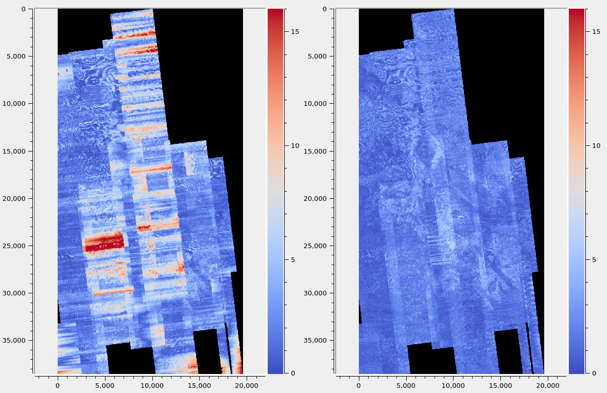
Fig. 16.10 Mosaicked triangulation error image (Section 14.6.1), before
(left) and after (right) solving for jitter. The range of values is between 0
and 15 meters. It can be seen that the triangulation error greatly decreases.
This was produced with dem_mosaic --max.
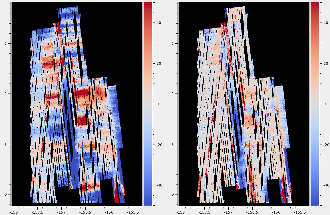
Fig. 16.11 Signed difference of the mosaicked DEM and MOLA before (left) and after (right) solving for jitter. It can be seen that the jitter artifacts are greatly attenuated. Some systematic error is seen in the vertical direction, roughly in the middle of the image. It is in the area where the MOLA data is sparsest, and maybe that results in the ground constraint not working as well. Or could be related to the seams issue noted earlier.
16.38.9. Example 2: WorldView-3 DigitalGlobe images on Earth
Jitter was successfully solved for a pair of WorldView-3 images over a mountainous site in Grand Mesa, Colorado, US.
This is a much more challenging example than the earlier one for CTX, because:
Images are much larger, at 42500 x 71396 pixels, compared to 5000 x 52224 pixels for CTX.
The jitter appears to be at much higher frequency, necessitating using 50 image lines for each position and orientation to optimize rather than 1000.
Many dense interest point matches and anchor points are needed to capture the high-frequency jitter. Many anchor points are needed to prevent the solution from becoming unstable at earlier and later image lines.
The terrain is very steep, which introduces some extraneous signal in the problem to optimize.
See Section 16.38.1 regarding limitations of this program.
We consider a dataset with two images named 1.tif and 2.tif, and corresponding camera files 1.xml and 2.xml, having the exact DigitalGlobe linescan model.
16.38.9.1. Bundle adjustment
Bundle adjustment was invoked first to reduce any errors between the cameras. This is not strictly necessary for WorldView images, as they are usually quite well-registered.
This command expects raw (not mapprojected) images:
bundle_adjust \
-t dg \
--ip-detect-method 1 \
--ip-per-image 10000 \
--tri-weight 0.1 \
--tri-robust-threshold 0.1 \
--camera-weight 0 \
--remove-outliers-params '75.0 3.0 10 10' \
1.tif 2.tif \
1.xml 2.xml \
-o ba/run
A lot of interest points were used, and the outlier filter threshold was generous, since, because of trees and shadows in the images, likely some interest points may not be too precise but they could still be good.
16.38.9.2. Mapprojection
Because of the steep terrain, the images were mapprojected onto the
Copernicus 30 m DEM (Section 6.1.7.1). We name that DEM
ref.tif. (Ensure the DEM is relative to WGS84 and not EGM96,
and convert if necessary; see Section 6.1.7.2.)
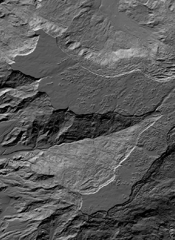
Fig. 16.12 The Copernicus 30 DEM for the area of interest. Some of the topographic signal, including cliff edges and trees will be noticeable in the error images produced below.
Mapprojection of the two images (Section 6.1.7):
proj="+proj=utm +zone=13 +datum=WGS84 +units=m +no_defs"
for i in 1 2; do
mapproject -t dg \
--nodes-list nodes_list.txt \
--tr 0.4 \
--t_srs "$proj" \
ref.tif ${i}.tif ${i}.xml ${i}.map.tif
done
Here the exact cameras were used for mapprojection (option -t dg). In
earlier versions of ASP this was slow, and the faster RPC model
was used (-t rpc).
Here we did not use the adjustments from bundle_adjust,
as it appears that the original cameras are already quite accurate.
We will incorporate those into subsequent steps, however.
16.38.9.3. Stereo
Stereo was done with the asp_mgm algorithm. We found that the option
--subpixel-mode 1 may result in somewhat more accurate interest point
matches from disparity (for use later) but --subpixel-mode 9 could produce a
terrain model with fewer artifacts. This likely needs more study. We will proceed
with --subpixel-mode 1 here. Subpixel mode 3 (or 2) would likely be better
than any of these, but are a lot slower.
It also appears that it is preferable to use mapprojected images than some other alignment methods as those would result in more subpixel artifacts which would obscure the jitter signal which we will solve for.
The option --max-disp-spread 100 was used because the images
had many clouds (Section 5.4).
A large number of dense interest point matches from stereo disparity will be created (Section 16.38.5), to be used later to solve for jitter.
parallel_stereo \
--max-disp-spread 100 \
--nodes-list nodes_list.txt \
--ip-per-image 10000 \
--stereo-algorithm asp_mgm \
--subpixel-mode 1 \
--processes 6 \
--alignment-method none \
--num-matches-from-disparity 60000 \
--bundle-adjust-prefix ba/run \
1.map.tif 2.map.tif 1.xml 2.xml \
run_1_2_map/run \
ref.tif
proj="+proj=utm +zone=13 +datum=WGS84 +units=m +no_defs"
point2dem --tr 0.4 --t_srs "$proj" --errorimage \
run_1_2_map/run-PC.tif
A discussion regarding the projection to use above is in Section 16.56.1.
16.38.9.4. Alignment
The alignment step is not strictly necessary for WorldView images, as they are rather well-aligned already. Here we show the step for completeness.
Align the stereo DEM to the reference DEM:
pc_align --max-displacement 100 \
run_1_2_map/run-DEM.tif ref.tif \
--save-inv-transformed-reference-points \
-o align/run
proj="+proj=utm +zone=13 +datum=WGS84 +units=m +no_defs"
point2dem --tr 0.4 --t_srs "$proj" align/run-trans_reference.tif
It is suggested to hillshade and inspect the obtained DEM and overlay
it onto the hillshaded reference DEM. The geodiff command
(Section 16.26) can be used to take their difference.
Apply the alignment transform to the bundle-adjusted cameras, to align them with the reference terrain:
bundle_adjust \
--input-adjustments-prefix ba/run \
--match-files-prefix ba/run \
--skip-matching \
--initial-transform align/run-inverse-transform.txt \
1.tif 2.tif 1.xml 2.xml \
--apply-initial-transform-only \
-o align/run
If the clouds in pc_align were in reverse order, the direct transform must
be used, not the inverse (Section 16.53.14).
16.38.9.5. Solving for jitter
Copy the produced dense interest point matches for use in solving for jitter:
mkdir -p dense
cp run_1_2_map/run-disp-1.map__2.map.match \
dense/run-1__2.match
In ASP 3.4.0 or later, that file to be copied is named instead
run_1_2_map/run-disp-1__2.match, or so, reflecting the names of the raw
images, as these matches are between the original images, even if produced
from mapprojected images.
Instead of copying and renaming, these matches can be passed with
--match-files-prefix run_1_2_map/run-disp, reusing the existing prefix. It is
suggested to not rename match files when the image names are long, as that can
invalidate the shortening of long match file names (Section 19.11).
See Section 16.38.5 for a longer explanation regarding dense and sparse interest point matches.
Solve for jitter. This command expects raw (not mapprojected) images:
jitter_solve \
1.tif 2.tif \
1.xml 2.xml \
--input-adjustments-prefix align/run \
--match-files-prefix dense/run \
--num-iterations 50 \
--max-pairwise-matches 100000 \
--max-initial-reprojection-error 20 \
--camera-position-uncertainty 1000,1000 \
--tri-weight 0.1 \
--tri-robust-threshold 0.1 \
--num-lines-per-position 400 \
--num-lines-per-orientation 400 \
--heights-from-dem ref.tif \
--heights-from-dem-uncertainty 10 \
--num-anchor-points 10000 \
--num-anchor-points-extra-lines 500 \
--anchor-dem ref.tif \
--anchor-dem-uncertainty 50 \
-o jitter/run
The value of --heights-from-dem-uncertainty is very important. See
Section 16.38.2.2 regarding the DEM constraint,
Section 16.38.3 regarding camera constraints, and
Section 16.38.6 regarding anchor points.
The report files mentioned in Section 16.38.17 can be very helpful in evaluating how well the jitter solver worked, even before rerunning stereo.
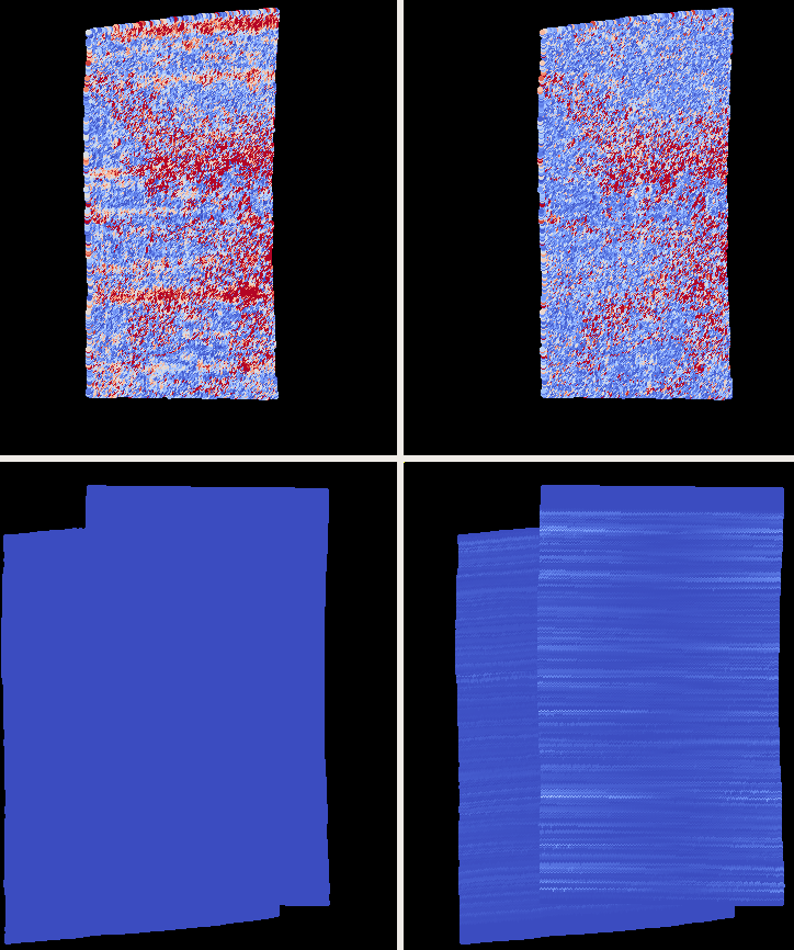
Fig. 16.13 The pixel reprojection errors per triangulated point (first column) and per anchor point (second column) before and after (left and right) solving for jitter. Blue shows an error of 0, and red is an error of at least 0.3 pixels.
It can be seen in Fig. 16.13 that after optimization the jitter (oscillatory pattern) goes away, but the errors per anchor point do not increase much. The remaining red points are because of the steep terrain. See Section 16.38.17 for description of these output files and how they were plotted.
16.38.9.6. Redoing mapprojection and stereo
The jitter solver produces optimized CSM cameras (Section 8.12), for all types of input cameras.
One can reuse the previously created mapprojected images with the new cameras (Section 16.38.9.7). Alternatively, here is how to recreate the mapprojected images:
proj="+proj=utm +zone=13 +datum=WGS84 +units=m +no_defs"
for i in 1 2; do
mapproject -t csm \
--nodes-list nodes_list.txt \
--tr 0.4 --t_srs "$proj" \
ref.tif ${i}.tif \
jitter/run-${i}.adjusted_state.json \
${i}.jitter.map.tif
done
Run stereo:
parallel_stereo \
--max-disp-spread 100 \
--nodes-list nodes_list.txt \
--ip-per-image 20000 \
--stereo-algorithm asp_mgm \
--subpixel-mode 9 \
--processes 6 \
--alignment-method none \
1.jitter.map.tif 2.jitter.map.tif \
jitter/run-1.adjusted_state.json \
jitter/run-2.adjusted_state.json \
stereo_jitter/run \
ref.tif
point2dem --tr 0.4 --t_srs "$proj" \
--errorimage \
stereo_jitter/run-PC.tif
16.38.9.7. Reusing a previous run
In ASP 3.3.0 or later, the mapprojection need not be redone, and stereo can resume at the triangulation stage (Section 6.1.7.8). This saves a lot of computing. The commands in the previous section can be replaced with:
parallel_stereo \
--max-disp-spread 100 \
--nodes-list nodes_list.txt \
--ip-per-image 20000 \
--stereo-algorithm asp_mgm \
--subpixel-mode 9 \
--processes 6 \
--alignment-method none \
--prev-run-prefix run_1_2_map/run \
1.map.tif 2.map.tif \
jitter/run-1.adjusted_state.json \
jitter/run-2.adjusted_state.json \
stereo_jitter/run \
ref.tif
point2dem --tr 0.4 --t_srs "$proj" \
--errorimage \
stereo_jitter/run-PC.tif
Note how we used the old mapprojected images 1.map.tif and 2.map.tif,
the option --prev-run-prefix pointing to the old run, while the
triangulation is done with the new jitter-corrected CSM cameras.
16.38.9.8. Validation
The geodiff command (Section 16.26) can be used to take the absolute difference of the aligned DEM before jitter correction and the one after it:
geodiff --float --absolute align/run-trans_reference-DEM.tif \
stereo_jitter/run-DEM.tif -o stereo_jitter/run
See Fig. 16.14 for results.
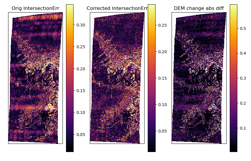
Fig. 16.14 The colorized triangulation error (Section 14.6.1) before and after solving for jitter, and the absolute difference of the DEMs before and after solving for jitter (left-to-right). It can be seen that the oscillatory pattern in the intersection error is gone, and the DEM changes as a result. The remaining signal is due to the steep terrain, and is rather small.
16.38.10. Example 3: Airbus Pleiades
In this section we will solve for jitter with Pleiades linescan cameras. The same approach applies to SPOT 6/7 (Section 8.27) and PeruSat-1 (Section 8.24). SPOT 6/7 and PeruSat-1 support is available as of build 2026/03 (Section 2.1).
We will investigate the effects of two kinds of ground constraints:
--tri-weight and --heights-from-dem (Section 16.38.2). The first
constraint tries to keep the triangulated points close to where they are, and
the second tries to tie them to a reference DEM. Note that if these are used
together, the first one will kick in only in regions where there is no coverage
in the provided DEM.
The conclusion is that if the two kinds of ground constraints are weak, and the reference DEM is decent, the results are rather similar. The DEM constraint is preferred if a good reference DEM is available, and the cameras are aligned to it.
See Section 16.38.1 regarding limitations of this program.
16.38.10.1. Creation of terrain model
The site used is Grand Mesa, as in Section 16.38.9, and the two recipes also have similarities.
First, a reference DEM (Copernicus) for the area is fetched, and
adjusted to be relative to WGS84, creating the file ref-adj.tif
(Section 6.1.7.1).
Let the images be called 1.tif and 2.tif. The Pleiades exact camera
model names usually start with the prefix DIM. Here, for simplicity, we will
name them 1.xml and 2.xml.
Do not use the Pleiades RPC camera models. Their names start with the PRC
prefix.
Since the GSD specified in these files is about 0.72 m, this value is used in mapprojection of both images (Section 6.1.7):
proj="+proj=utm +zone=13 +datum=WGS84 +units=m +no_defs"
mapproject --processes 4 --threads 4 \
--tr 0.72 --t_srs "$proj" \
--nodes-list nodes_list.txt \
ref-adj.tif 1.tif 1.xml 1.map.tif
and same for the other image.
Since the two mapprojected images agree very well with the hillshaded
reference DEM when overlaid in stereo_gui (Section 16.72),
no bundle adjustment was used.
Stereo was run, and we create dense interest point matches from disparity, that will be needed later:
outPrefix=stereo_map_12/run
parallel_stereo \
--max-disp-spread 100 \
--nodes-list nodes_list.txt \
--ip-per-image 10000 \
--num-matches-from-disparity 90000 \
--stereo-algorithm asp_mgm \
--subpixel-mode 9 \
--processes 6 \
--alignment-method none \
1.map.tif 2.map.tif \
1.xml 2.xml \
$outPrefix \
ref-adj.tif \
DEM creation:
proj="+proj=utm +zone=13 +datum=WGS84 +units=m +no_defs"
point2dem --t_srs "$proj" \
--errorimage \
${outPrefix}-PC.tif
See Section 16.56.1 for a discussion of the projection to use.
Colorize the triangulation (ray intersection) error, and create some image pyramids for inspection later:
colormap --min 0 --max 1.0 ${outPrefix}-IntersectionErr.tif
stereo_gui --create-image-pyramids-only \
--hillshade ${outPrefix}-DEM.tif
stereo_gui --create-image-pyramids-only \
${outPrefix}-IntersectionErr_CMAP.tif
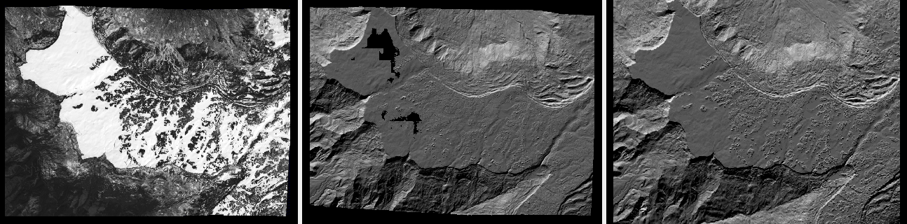
Fig. 16.15 Left to right: One of the input images, the produced hillshaded DEM, and the reference Copernicus DEM.
It can be seen in Fig. 16.15 (center) that a small portion having snow failed to correlate. That is not a showstopper here. Perhaps adjusting the image normalization options in Section 17 may resolve this.
16.38.10.2. Correcting the jitter
The jitter can clearly be seen in Fig. 16.16 (left).
There seem to be about a dozen oscillations. Hence, jitter_solve
will be invoked with one position and orientation sample for each 500
image lines, which results in about 100 samples for these, along the
satellite track. Note that earlier we used
--num-matches-from-disparity 90000 which created about 300 x
300 dense interest point matches for these roughly square input
images. These numbers usually need to be chosen with some care.
Copy the dense interest point matches found in stereo, using the convention
(Section 16.5.10.1) expected later by jitter_solve:
mkdir -p matches
/bin/cp -fv stereo_map_12/run-disp-1.map__2.map.match \
matches/run-1__2.match
In ASP 3.4.0 or later, that file to be copied is named instead
run_1_2_map/run-disp-1__2.match, or so, reflecting the names of the raw
images. Then, instead of copying and renaming, these matches can be passed with
--match-files-prefix stereo_map_12/run-disp, reusing the existing prefix. It
is suggested to not rename match files when the image names are long, as that can
invalidate the shortening of long match file names (Section 19.11).
See Section 16.38.5 for a longer explanation regarding dense interest point matches.
Solve for jitter with the intrinsic --tri-weight ground constraint
(Section 16.38.2). Normally, the cameras should be bundle-adjusted and
aligned to the reference DEM, and then below the option
--input-adjustments-prefix should be used, but in this case the initial
cameras were accurate enough, so these steps were skipped.
jitter_solve \
1.tif 2.tif \
1.xml 2.xml \
--match-files-prefix matches/run \
--num-iterations 50 \
--max-pairwise-matches 100000 \
--max-initial-reprojection-error 20 \
--camera-position-uncertainty 1000,1000 \
--tri-weight 0.1 \
--tri-robust-threshold 0.1 \
--num-lines-per-position 500 \
--num-lines-per-orientation 500 \
--num-anchor-points 10000 \
--num-anchor-points-extra-lines 500 \
--anchor-dem ref-adj.tif \
--anchor-dem-uncertainty 50 \
-o jitter_tri/run
See Section 16.38.3 for a discussion of camera constraints. See Section 16.38.6 regarding anchor points.
The report files mentioned in Section 16.38.17 can be very helpful in evaluating how well the jitter solver worked, even before rerunning stereo.
Next, we invoke the solver with the same initial data, but with a constraint
tying to the reference DEM, with the option --heights-from-dem ref-adj.tif.
Since the difference between the created stereo DEM and the reference DEM is on
the order of 5-10 meters, we will use --heights-from-dem-uncertainty 20.
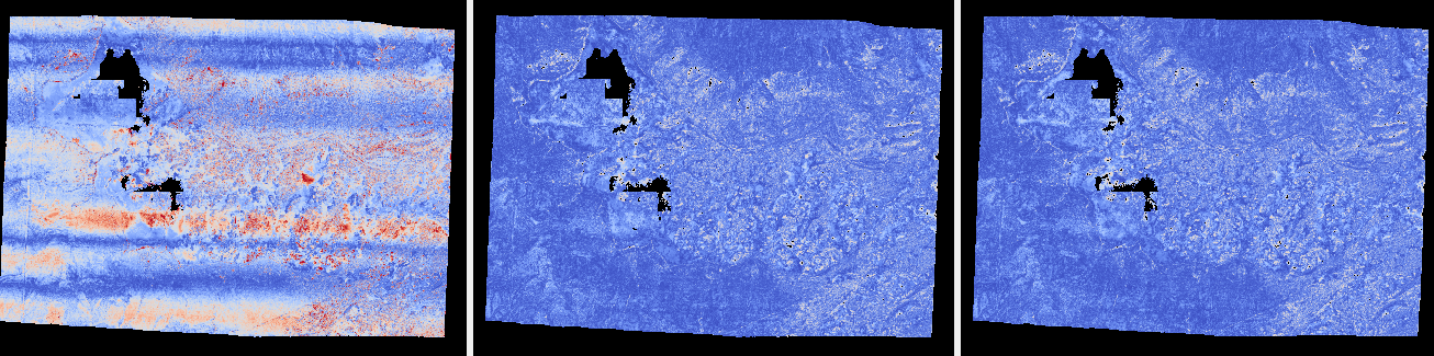
Fig. 16.16 Stereo intersection error (Section 14.6.1)
before solving for jitter (left),
after solving for it with the --tri-weight constraint (middle)
and with the --heights-from-dem constraint (right). Blue = 0
m, red = 1 m.
It can be seen in Fig. 16.16 that any of these constraints can work at eliminating the jitter.
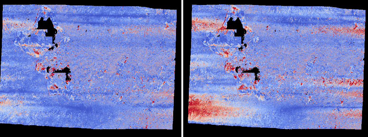
Fig. 16.17 Absolute difference of the stereo DEMs before and after
solving for jitter. Left: with the --tri-weight
constraint. Right: with the --heights-from-dem constraint. Blue
= 0 m, red = 1 m.
It is very instructive to examine how much the DEM changed as a result. It can be seen in Fig. 16.17 that the reference DEM constraint changes the result more. Likely, a smaller value of the weight for that constraint could have been used.
16.38.11. ASTER cameras
ASTER (Section 8.21) is a very good testbed for studying jitter because there are millions of free images over a span of 20 years, with many over the same location, and the images are rather small, on the order of 4,000 - 5,000 pixels along each dimension.
See Section 16.38.1 regarding limitations of this program.
16.38.11.1. Setup
In this example we worked on a rocky site in Egypt with a latitude 24.03562 degrees and longitude of 25.85006 degrees. Dozens of cloud-free stereo pairs are available here. The jitter pattern, including its frequency, turned out to be quite different in each stereo pair we tried, but the solver was able to minimize it in all cases.
Fetch and prepare the data as documented in Section 8.21.1. Here we will
work with dataset AST_L1A_00301062002090416_20231023221708_3693.
A reference Copernicus DEM can be downloaded per Section 6.1.7.1. Use
dem_geoid to convert the DEM to be relative to WGS84.
16.38.11.2. Initial stereo and alignment
We will call the two images in an ASTER stereo pair out-Band3N.tif and
out-Band3B.tif. This is the convention used by aster2asp
(Section 16.2), and instead of out any other string can be used. The
corresponding cameras are out-Band3N.xml and out-Band3B.xml. The
reference Copernicus DEM relative to WGS84 is ref.tif.
Bundle adjustment:
bundle_adjust -t aster \
--camera-weight 0.0 \
--tri-weight 0.1 \
--tri-robust-threshold 0.1 \
--num-iterations 50 \
out-Band3N.tif out-Band3B.tif \
out-Band3N.xml out-Band3B.xml \
-o ba/run
Not using -t aster will result in RPC cameras being used, which would lead
to wrong results. The adjusted cameras are saved in CSM format
(Section 8.12.6), which is needed for the jitter solver. The produced
.adjust files should not be used as they save the adjustments only.
Stereo was done with mapprojected images. The reference DEM was blurred a little as it is at the resolution of the images, and then any small misalignment between the images and the DEM may result in artifacts:
dem_mosaic --dem-blur-sigma 2 ref.tif -o ref_blur.tif
Mapprojection in local stereographic projection:
proj='+proj=stere +lat_0=24.0275 +lon_0=25.8402 +k=1 +x_0=0 +y_0=0 +datum=WGS84 +units=m +no_defs'
mapproject -t csm \
--tr 15 --t_srs "$proj" \
ref_blur.tif out-Band3N.tif \
ba/run-out-Band3N.adjusted_state.json \
out-Band3N.map.tif
The same command is used for the other image. Both must use the same resolution
in mapprojection (option --tr).
It is suggested to overlay and inspect in stereo_gui (Section 16.72)
the produced images and the reference DEM and check for any misalignment or
artifacts. ASTER is quite well-aligned to the reference DEM.
Stereo with mapprojected images (Section 6.1.7) and DEM generation
is run. Here the asp_mgm algorithm is not used as it smears the jitter
signal:
parallel_stereo \
--stereo-algorithm asp_bm \
--subpixel-mode 1 \
--max-disp-spread 100 \
--num-matches-from-disparity 100000 \
out-Band3N.map.tif out-Band3B.map.tif \
ba/run-out-Band3N.adjusted_state.json \
ba/run-out-Band3B.adjusted_state.json \
stereo_bm/run \
ref_blur.tif
point2dem --errorimage --t_srs "$proj" \
--tr 15 stereo_bm/run-PC.tif \
--orthoimage stereo_bm/run-L.tif
We chose to use option --num-matches-from-disparity to create a large and
uniformly distributed set of interest point matches. That is necessary because
the jitter that we will solve for has rather high frequency.
See Section 16.56.1 for a discussion of the projection to use in DEM creation.
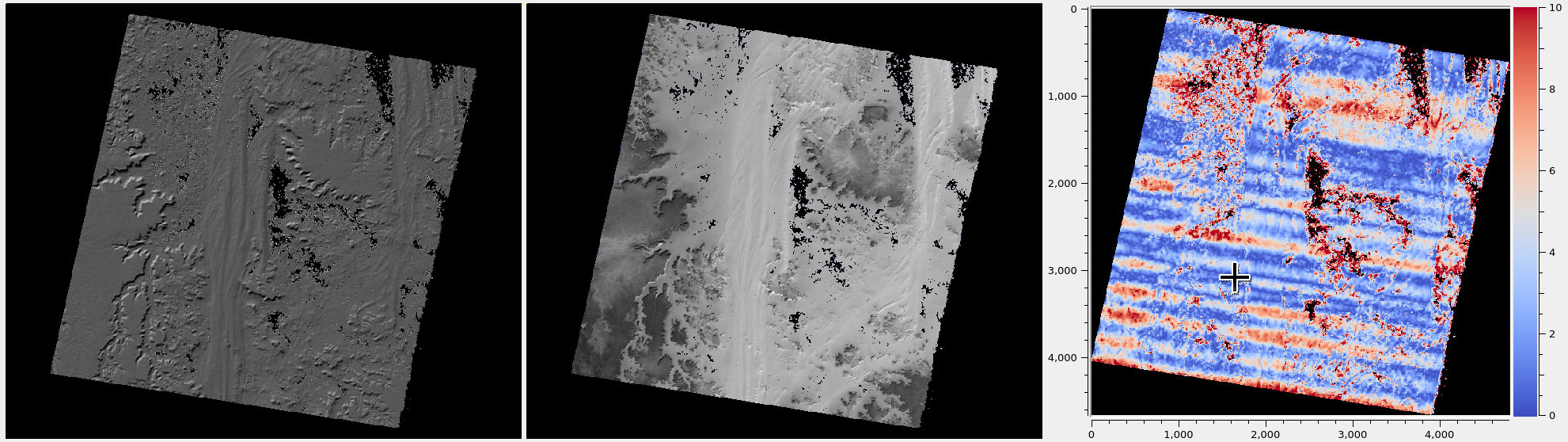
Fig. 16.18 Produced DEM, orthoimage and intersection error. The correlation algorithm has some trouble over sand, resulting in holes. The jitter is clearly visible, and will be solved for next. The color scale on the right is from 0 to 10 meters.
The created DEM is brought in the coordinate system of the reference DEM. This results in a small shift in this case, but it is important to do this each time before solving for jitter.
  pc_align --max-displacement 50          \
  stereo_bm/run-DEM.tif ref.tif           \
  -o stereo_bm/run-align                  \
  --save-inv-transformed-reference-points

point2dem --t_srs "$proj" --tr 15 \
  stereo_bm/run-align-trans_reference.tif
One has to be careful with the value of --max-displacement that is used
(Section 16.53).
Take the difference with the reference DEM after alignment:
geodiff stereo_bm/run-align-trans_reference-DEM.tif \
  ref.tif -o stereo_bm/run
The result of this is shown in Fig. 16.21. Apply the alignment transform to the cameras (Section 16.53.14):
bundle_adjust -t csm                        \
  --initial-transform                       \
  stereo_bm/run-align-inverse-transform.txt \
  --apply-initial-transform-only            \
  out-Band3N.map.tif out-Band3B.map.tif     \
  ba/run-out-Band3N.adjusted_state.json     \
  ba/run-out-Band3B.adjusted_state.json     \
  -o ba_align/run
This will create new cameras in CSM format in the directory ba_align.
It is important to use here the inverse alignment transform, as we want to map
from the stereo DEM to the reference DEM, and the forward transform would do the
opposite, given how pc_align was invoked.
If the produced difference of DEMs shows large residuals consistent with the terrain, one should consider applying more blur to the reference terrain and/or redoing mapprojection and stereo with the now-aligned cameras, and see if this improves this difference.
16.38.11.3. Solving for jitter
Copy the dense match file (Section 12.2.4.2) to follow the naming convention for unprojected (original) images:
mkdir -p jitter
cp stereo_bm/run-disp-out-Band3N.map__out-Band3B.map.match \
  jitter/run-out-Band3N__out-Band3B.match
In ASP 3.4.0 or later, that file to be copied is named instead
run_1_2_map/run-disp-out-Band3N__out-Band3B.match, or so, reflecting the names
of the raw images. Then, instead of copying and renaming, these matches can be
passed with --match-files-prefix stereo_bm/run-disp, reusing the existing
prefix. It is suggested to not rename match files when the image names are long,
as that can invalidate the shortening of long match file names
(Section 19.11).
The naming convention for the match files is:
<prefix>-<image1>__<image2>.match
where the image names are without the directory name and extension (Section 16.5.10.1). See Section 16.38.5 for more information on interest point matches.
Here it is important to use a lot of match points and a low
value for --num-lines-per-orientation and same for position,
because the jitter has rather high frequency.
Solve for jitter with the aligned cameras:
jitter_solve out-Band3N.tif out-Band3B.tif        \
  ba_align/run-run-out-Band3N.adjusted_state.json \
  ba_align/run-run-out-Band3B.adjusted_state.json \
  --max-pairwise-matches 100000                   \
  --num-lines-per-position 100                    \
  --num-lines-per-orientation 100                 \
  --max-initial-reprojection-error 20             \
  --num-iterations 50                             \
  --match-files-prefix jitter/run                 \
  --heights-from-dem ref.tif                      \
  --heights-from-dem-uncertainty 20               \
  --num-anchor-points 0                           \
  -o jitter/run
The DEM uncertainty constraint was set to 20, as the image GSD is 15 meters. A higher value for the uncertainty is recommended, such as 200 or more, if the reference DEM has large systematic differences with the stereo DEM. A tight uncertainty constraint can result in unphysical oscillations in the terrain model.
Here, --num-lines-per-position and --num-lines-per-orientation are quite
low. This may result in high-frequency oscillations in the produced DEM. If so,
these need to be increased by 2x or 4x.
See Section 16.38.3 for a discussion of camera constraints, and Section 16.38.6 regarding anchor points.
The report files mentioned in Section 16.38.17 can be very helpful in evaluating how well the jitter solver worked, even before rerunning stereo.
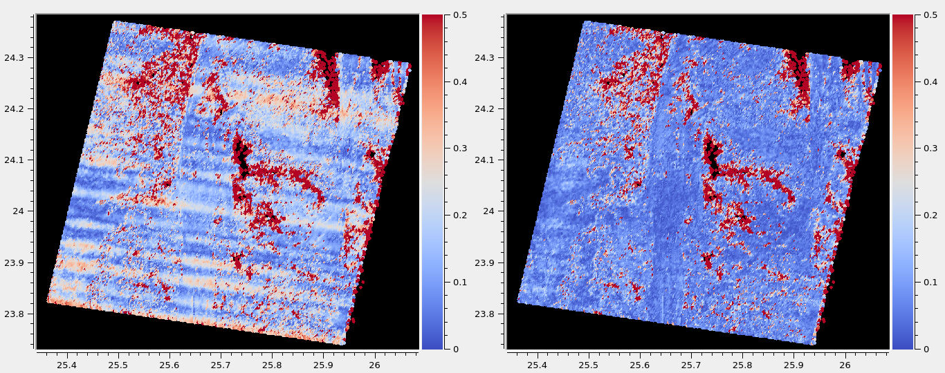
Fig. 16.19 Pixel reprojection errors (Section 16.38.17) before (left) and after (right) solving for jitter. Compare with the ray intersection error in Fig. 16.20.
Then, mapproject, parallel_stereo and point2dem can be run again,
with the new cameras created in the jitter directory.
Do not reuse the previous stereo run. So, do not use the option
--prev-run-prefix. This introduces artifacts in the DEM. Likely it is
because the cameras changed too much. It is suggested to re-mapproject with the
optimized cameras, and re-run stereo from scratch.
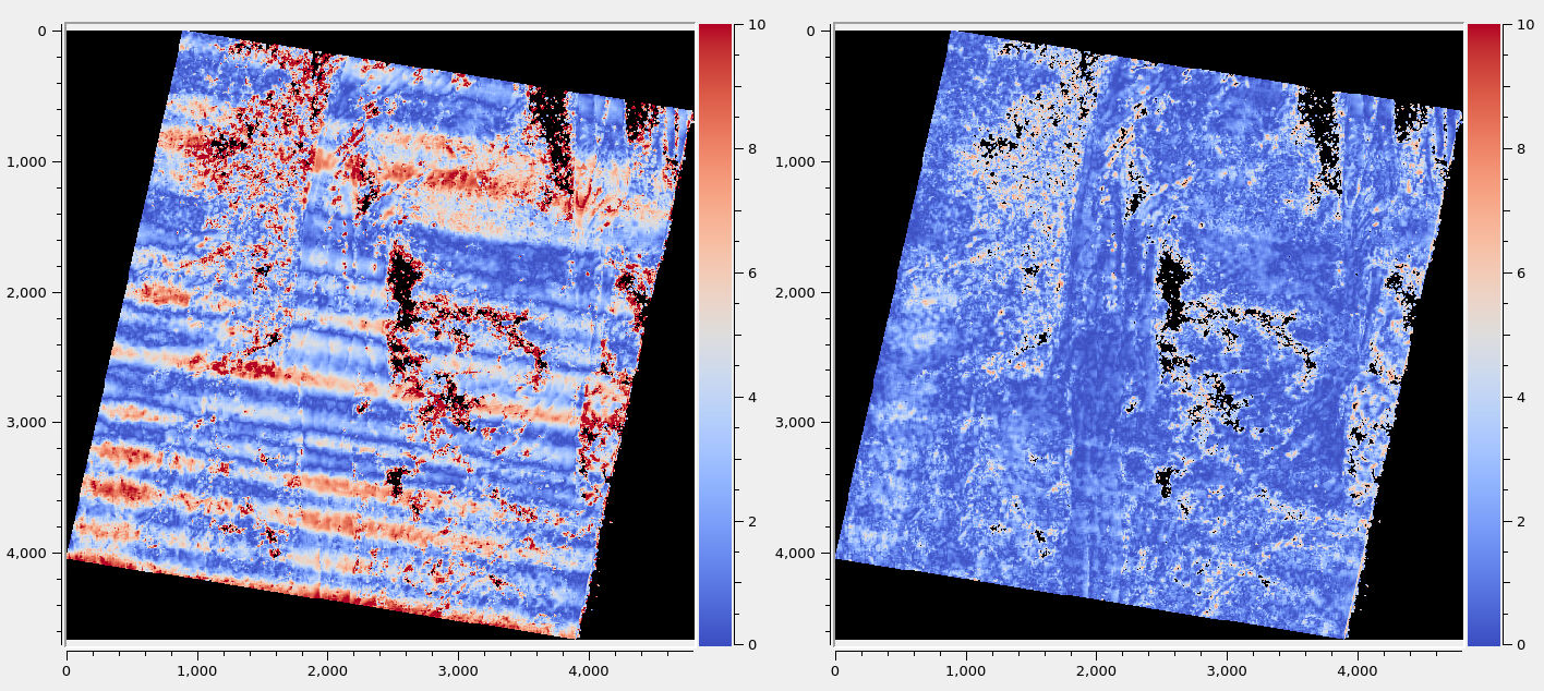
Fig. 16.20 The ray intersection error before (left) and after (right) solving for jitter. The scale is in meters. Same pattern is seen as for the pixel reprojection errors earlier.
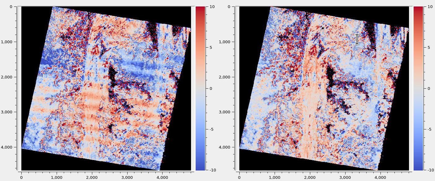
Fig. 16.21 The signed difference between the ASP DEM and the reference DEM, before (left) and after (right) solving for jitter. The scale is in meters. It can be seen that the jitter pattern is gone.
16.38.12. Jitter with synthetic cameras and orientation constraints
The effectiveness of jitter_solve can be validated using synthetic data,
when we know what the answer should be ahead of time. The synthetic data can
be created with sat_sim (Section 16.62). See a recipe in
Section 16.62.7.
For example, one may create three linescan images and cameras, using various values for the pitch angle, such as -30, 0, and 30 degrees, modeling a camera that looks forward, down, and aft. One can choose to not have any jitter in the images or cameras, then create a second set of cameras with pitch (along-track) jitter.
Then, jitter_solve can be used to solve for the jitter. It can be invoked
with the images not having jitter and the cameras having the jitter.
It is suggested to use the roll and yaw constraints (--roll-weight and
--yaw-weight, with values on the order of 1e+4), to keep these angles in
check while correcting the pitch jitter. Note that with non-synthetic cameras,
one needs to add the --initial-camera-constraint option.
The --heights-from-dem option should be used as well, to tie the solution to
the reference DEM.
We found experimentally that, if the scan lines for all the input cameras are perfectly parallel, then the jitter solver will not converge to the known solution. This is because the optimization problem is under-constrained. If the scan lines for different cameras meet at, for example, a 6-15 degree angle, and the lines are long enough to offer good overlap, then the “rigidity” of a given scan line will be able to help correct the jitter in the scan lines for the other cameras intersecting it, resulting in a solution close to the expected one.
See a worked-out example for how to set orientation constraints in Section 16.38.14. There, frame cameras are used as well, to add “rigidity” to the setup.
16.38.13. Constraining direction of jitter with real cameras
For synthetic cameras created with sat_sim (Section 16.62), it is
assumed that the orbit is a straight segment in projected coordinates (hence
an ellipse if the orbit end points are at the same height above the datum). It
is also assumed that such a camera has a fixed roll, pitch, and yaw relative to
the satellite along-track / across-track directions, with jitter added to these
angles (Section 16.62.4, and Section 16.62.6).
For a real linescan satellite camera, the camera orientation is variable and not
correlated to the orbit trajectory. The jitter_solve program can then
constrain each camera sample being optimized not relative to the orbit
trajectory, but relative to initial camera orientation for that sample.
That is accomplished by invoking the jitter solver as in
Section 16.38.12, with the additional option
--initial-camera-constraint. See the description of this option in
Section 16.38.18.
This option is very experimental and its effectiveness was only partially validated. If having a rig, it is suggested to employ instead the strategy in Section 16.38.15.
This option can be used with synthetic cameras as well. The results then will be somewhat different than without this option, especially towards orbit end points, where the overlap with other cameras is small.
16.38.14. Mixing linescan and frame cameras
This solver allows solving for jitter using a combination of linescan and frame (pinhole) cameras, if both of these are stored in the CSM format (Section 8.12). How to convert existing cameras to this format is described in Section 16.8.1.4 and Section 16.8.1.7.
For now, this functionality was validated only with synthetic cameras created
with sat_sim (Section 16.62). In this case, roll and yaw constraints for
the orientations of cameras being optimized are supported, for both linescan and
frame cameras.
When using real data, it is important to ensure they are acquired at close-enough times, with similar illumination and ground conditions (such as snow thickness).
Here is a detailed recipe.
Consider a DEM named dem.tif, and an orthoimage named ortho.tif. Let x
be a column index in the DEM and y1 and y2 be two row indices. These
will determine the path on the ground seen by the satellite. Let h be the
satellite height above the datum, in meters. Set, for example:
x=4115
y1=38498
y2=47006
h=501589
opt="--dem dem.tif
  --ortho ortho.tif
  --first $x $y1 $h
  --last  $x $y2 $h
  --first-ground-pos $x $y1
  --last-ground-pos  $x $y2
  --frame-rate 45
  --jitter-frequency 5
  --focal-length 551589
  --optical-center 2560 2560
  --image-size 5120 5120
  --velocity 7500
  --save-ref-cams"
Create nadir-looking frame images and cameras with no jitter:
sat_sim $opt                  \
  --save-as-csm               \
  --sensor-type pinhole       \
  --roll 0 --pitch 0 --yaw 0  \
  --horizontal-uncertainty    \
  "0.0 0.0 0.0"               \
  --output-prefix jitter0.0/n
Create a forward-looking linescan image and camera, with no jitter:
sat_sim $opt                  \
  --sensor-type linescan      \
  --roll 0 --pitch 30 --yaw 0 \
  --horizontal-uncertainty    \
  "0.0 0.0 0.0"               \
  --output-prefix jitter0.0/f
Create a forward-looking linescan camera, with no images, with pitch jitter:
sat_sim $opt                  \
  --no-images                 \
  --sensor-type linescan      \
  --roll 0 --pitch 30 --yaw 0 \
  --horizontal-uncertainty    \
  "0.0 2.0 0.0"               \
  --output-prefix jitter2.0/f
The tool cam_test (Section 16.9) can be run to compare the camera
with and without jitter:
cam_test --session1 csm    \
  --session2 csm           \
  --image jitter0.0/f.tif  \
  --cam1  jitter0.0/f.json \
  --cam2  jitter2.0/f.json
This will show that projecting a pixel from the first camera to the ground and then projecting it back to the second camera will result in around 2 pixels of discrepancy, which makes sense given the horizontal uncertainty set above and the fact that our images are at around 0.9 m/pixel ground resolution.
To reliably create reasonably dense interest point matches between the frame and linescan images, first mapproject (Section 16.41) them:
for f in jitter0.0/f.tif                    \
         jitter0.0/n-1[0-9][0-9][0-9][0-9].tif; do
    g=${f/.tif/} # remove .tif
    mapproject --tr 0.9                     \
      dem.tif ${g}.tif ${g}.json ${g}.map.tif
done
This assumes that the DEM is in a local projection in units of meter. Otherwise
the --t_srs option should be set.
Create the lists of images, cameras, then a list for the mapprojected images and
the DEM. We use individual ls commands to avoid the inputs being reordered:
dir=ba
mkdir -p $dir
ls jitter0.0/f.tif                        >  $dir/images.txt
ls jitter0.0/n-1[0-9][0-9][0-9][0-9].tif  >> $dir/images.txt

ls jitter0.0/f.json                       >  $dir/cameras.txt
ls jitter0.0/n-1[0-9][0-9][0-9][0-9].json >> $dir/cameras.txt

ls jitter0.0/f.map.tif                       >  $dir/map_images.txt
ls jitter0.0/n-1[0-9][0-9][0-9][0-9].map.tif >> $dir/map_images.txt
ls dem.tif                                   >> $dir/map_images.txt
Run bundle adjustment to get interest point matches:
parallel_bundle_adjust                           \
    --processes 10                               \
    --nodes-list nodes_list.txt                  \
    --num-iterations 50                          \
    --ip-detect-method 1                         \
    --tri-weight 0.1                             \
    --camera-weight 0                            \
    --auto-overlap-params "dem.tif 15"           \
    --min-matches 5                              \
    --remove-outliers-params '75.0 3.0 10 10'    \
    --min-triangulation-angle 5.0                \
    --ip-per-tile 500                            \
    --matches-per-tile 500                       \
    --max-pairwise-matches 6000                  \
    --image-list $dir/images.txt                 \
    --camera-list $dir/cameras.txt               \
    --mapprojected-data-list $dir/map_images.txt \
    -o ba/run
Here we assumed a minimum triangulation convergence angle of 5 degrees between
the two sets of cameras (Section 8.1). See Section 8.20 for
how to set up the computing nodes needed for --nodes-list.
We use --ip-detect-method 1 to detect interest points. This invokes the SIFT
feature detection method, which is more accurate than the default
--ip-detect-method 0. See Section 16.38.5 for more information on
interest point matches.
We could have used a ground constraint above, but since we only need the interest points and not the camera poses, it is not necessary. The default camera position constraint is also on (Section 16.38.3).
Solve for jitter with a ground constraint. Use roll and yaw constraints, to ensure movement only for the pitch angle:
jitter_solve                             \
    --num-iterations 50                  \
    --max-pairwise-matches 3000          \
    --clean-match-files-prefix           \
      ba/run                             \
    --roll-weight 10000                  \
    --yaw-weight 10000                   \
    --max-initial-reprojection-error 100 \
    --tri-weight 0.1                     \
    --tri-robust-threshold 0.1           \
    --num-anchor-points 10000            \
    --num-anchor-points-extra-lines 500  \
    --anchor-dem dem.tif                 \
    --anchor-dem-uncertainty 20          \
    --heights-from-dem dem.tif           \
    --heights-from-dem-uncertainty 10    \
    jitter0.0/f.tif                      \
    jitter0.0/n-images.txt               \
    jitter2.0/f.json                     \
    jitter0.0/n-cameras.txt              \
    -o jitter_solve/run
The value of --heights-from-dem-uncertainty should be chosen with care.
For non-synthetic cameras, one needs to add the option --initial-camera-constraint.
We used --max-pairwise-matches 3000 as the linescan camera has many
matches with each frame camera image, and there are many such frame camera
images. A much larger number would be used if we had only a couple of linescan
camera images and no frame camera images.
The initial cameras were not bundle-adjusted and aligned
to the reference DEM, as they were good enough. Normally one would
use them as input to jitter_solve with the option
--input-adjustments-prefix.
See Section 16.38.3 for a discussion of camera constraints.
Notice that the nadir-looking frame images are read from a list, in
jitter0.0/n-images.txt. This file is created by sat_sim. All the images
in such a list must be acquired in quick succession and be along the same
satellite orbit portion, as the trajectory of all these cameras will be used to
enforce the roll and yaw constraints.
A separate list must be created for each such orbital stretch, then added to the invocation above. The same logic is applied to the cameras for these images.
There is a single forward-looking image, but it is linescan, so there are many camera samples for it.
The forward-looking camera has jitter, so we used its version from the
jitter2.0 directory, not the one in jitter0.0.
This solver does not create anchor points for the frame cameras. There are usually many such images and they overlap a lot, so anchor points are not needed as much as for linescan cameras.
16.38.15. Rig constraints
This solver can model the fact that the input images have been acquired with one or more rigs. A rig can have one or more sensors. A sensor can be frame or linescan. Each rig can acquire several data collections. Each rig can have its own design.
16.38.15.1. Rig configuration
Each rig must have a designated reference sensor. The transforms from the reference sensor to other sensors on that rig will be optimized by this solver.
The intrinsics of all sensors for all rigs should be set in a single configuration file, in the format described in Section 16.60.4.
This solver assumes no lens distortion, no offsets between clocks of individual
sensors, and no depth measurements, so the entries for these in the rig
configuration file should be left at nominal values. The entries for
distorted_crop_size and undistorted_image_size should have the image
dimensions.
16.38.15.2. Assumptions
When a rig has both linescan and frame sensors, the reference sensor must be linescan. That is because the linescan sensor acquires image data more frequently.
The reference sensor must acquire pose readings frequently enough that pose interpolation in time is accurate. For a frame reference sensor, that may mean that all frame sensors acquire data simultaneously, or the reference sensor captures data at a finer rate than any observed jitter. For a linescan reference sensor, the parameters
--num-lines-per-positionand--num-lines-per-orientationneed to be smaller than 1/2 of the jitter period.The acquisition times of all sensors on a rig during a contiguous observation stretch must be within the time range of the reference sensor, to avoid extrapolation in time.
The acquisition times are known very accurately.
It is not assumed that acquisition times are synchronized between sensors, or that a frame camera has a fixed frame rate.
16.38.15.3. Naming convention
The images and cameras passed in must be in one-to-one correspondence.
The following format is expected for frame image and camera names:
<path>/<group><sep><timestamp><sep><sensor name>.<extension>
Any separator characters in <sep> must not contain alphanumeric
characters, as that will confuse the program. The timestamp must be
of the form <digits>.<digits> (no values such as 1e+7).
Example:
data/acq1_10000.23_sensor1.tif
All images acquired by a frame sensor in a given contiguous stretch of time must be listed in a text file of the form:
<path>/<group><sep><sensor name>.txt
which is passed in to the solver as an image file would be otherwise. The same applies to the cameras. An example is below.
Each linescan sensor image or camera name must be of the form:
<path>/<group><sep><sensor name>.<extension>
Each contiguous acquisition with a rig must have a unique group name, that will be part of all filenames produced at that time. In other words, acquisitions with different rigs or by the same rig at another time need to have different group names.
16.38.15.4. Example of sensors on a rig with a very small baseline
In this example we consider a rig with one linescan and one frame sensor. The rig looks straight down, so there is very little overall baseline between the sensors.
The linescan sensor acquires a single wide and tall image, while the frame camera records many rectangular images of much smaller dimensions. They both experience the same jitter.
The solver enforces the rig constraint between the sensors.
The frame camera images are shown to be able to help correct the jitter. That is because each frame camera image can serve as a template, relative to which oscillations in the linescan sensor can be measured.
The rig constraint is not essential here. This constraint is useful however when there are two sensors side-by-side, as then the rig helps constrain the yaw angle.
Synthetic data for this example can be produced as in Section 16.38.14, with the addition of modeling a rig, as in Section 16.62.8.
A straightforward application of the jitter-solving recipe in Section 16.38.14 will fail, as it is not possible to triangulate properly the points seen by the cameras, since the rays are almost parallel or slightly diverging. The following adjustments are suggested:
Use
--forced-triangulation-distance 500000for both bundle adjustment and jitter solving (the precise value here is not very important if the--heights-from-demconstraint is used, as the triangulated point will be adjusted based on the DEM). This will result in triangulated points even when the rays are parallel or a little divergent.Use
--min-triangulation-angle 1e-10in both bundle adjustment and jitter solving, to ensure we don’t throw away features with small convergence angle, as that will be almost all of them.Be generous with outlier filtering when there is a lot of jitter. Use, for example,
--remove-outliers-params '75.0 3.0 10 10'inbundle_adjustand--max-initial-reprojection-error 20injitter_solve.The option
--heights-from-demshould be used (Section 12.2.1.3).Use
--match-files-prefixinstead of--clean-match-files-prefixinjitter_solve, as maybe bundle adjustment filtered out too many good matches with a small convergence angle (if it was not invoked as suggested above).
Here’s the command for solving for jitter. This assumes interest points were
produced with bundle adjustment. It is preferred that they are dense, as in
previous sections. The same rig configuration can be used as when the input
images and cameras are created with sat_sim (Section 16.62.8).
jitter_solve                               \
    --rig-config rig.txt                   \
    --forced-triangulation-distance 500000 \
    --min-matches 1                        \
    --min-triangulation-angle 1e-10        \
    --num-iterations 50                    \
    --max-pairwise-matches 50000           \
    --match-files-prefix ba/run            \
    --max-initial-reprojection-error 100   \
    --num-anchor-points-per-tile 100       \
    --num-anchor-points-extra-lines 500    \
    --anchor-dem dem.tif                   \
    --anchor-dem-uncertainty 100           \
    --heights-from-dem dem.tif             \
    --heights-from-dem-uncertainty 10      \
    data/nadir_linescan.tif                \
    data/nadir_frame_images.txt            \
    data/nadir_linescan.json               \
    data/nadir_frame_cameras.txt           \
    -o jitter/run
The options --use-initial-rig-transforms, --fix-rig-rotations,
--fix-rig-translations, and --camera-position-uncertainty /
--camera-position-weight can constrain the solution in various ways. A rig
can be created by hand or generated by sat_sim to desired specifications
(Section 16.62.8).
The optimized rig will be saved in the output directory and can be inspected.
The value of --heights-from-dem-uncertainty can be decreased if the input DEM
is reliable and it is desired to tie the solution more to it.
When the linescan sensor is much wider than the frame sensor, the anchor points
should be constrained to the shared area of the produced images, to have the
same effect on both sensors. That is accomplished with the option
--anchor-weight-image.
It is important to examine the produced triangulated points and reprojection errors (Section 16.5.11.5) to ensure the points are well-distributed and that the errors are small and uniform.
The orbit_plot program (Section 16.44) can inspect the camera
orientations before and after optimization.
16.38.16. Point cloud constraint
In this scenario it is assumed that a reference point cloud is available that can constrain the jitter solution. The cloud can be in CSV format or a DEM. The cloud must be well-aligned with the input cameras. The cloud can be sparse.
This workflow requires having filtered stereo disparity files (F.tif,
Section 19) as made by parallel_stereo
(Section 16.51). For the moment, only a single stereo run is
supported.
The algorithm projects a reference terrain point into one camera, propagates it
through the stereo disparity to the other camera, and takes the pixel difference
with the direct projection in the other camera (this difference is called the
residual further down). The option --reference-terrain-uncertainty can set
the uncertainty, with a higher uncertainty resulting in less weight for this
constraint. The weight is also adjusted for the ground sample distance at each
reference terrain point.
The stereo runs should be produced either with the same images as invoked by the
jitter solver, or with mapprojected versions of those (the same order of images
need not be kept). The stereo run produces a file named {output prefix}-info.txt
that has some information which jitter_solve will use.
It is not important that the cameras or bundle-adjust prefixes passed to the jitter solving be the same as the ones for the stereo runs, but all the relevant files must be available, and the inputs to stereo must not be changed after the stereo runs are created.
The list of stereo prefixes (Section 3), should be set via
--stereo-prefix-list. The jitter solver will peek in those runs and figure
out how they relate to the images passed in to the solver. It will undo any
alignment or mapprojection transforms as appropriate.
This workflow does not preclude using the --heights-from-dem option or
anchor points. It assumes that no rig is present and that all cameras are
linescan.
If the images are mapprojected, this option loads fully in memory the DEM that
was used for mapprojecting them, for performance reasons, so it should not be
too large. Both mapprojected images must use the same DEM. The solver will not
fully load in memory the stereo disparity file (F.tif), but only portions as
needed.
Example usage:
echo {output prefix} > stereo_list.txt

jitter_solve                                    \
  --max-pairwise-matches 50000                  \
  --match-files-prefix ba/run                   \
  --num-iterations 50                           \
  --reference-terrain lidar.csv                 \
  --max-num-reference-points 50000              \
  --reference-terrain-uncertainty 10            \
  --csv-format 1:lon,2:lat,3:height_above_datum \
  --stereo-prefix-list stereo_list.txt          \
  --num-anchor-points-per-tile 50               \
  --num-anchor-points-extra-lines 1000          \
  --anchor-dem-uncertainty 10                   \
  --anchor-dem anchor_dem.tif                   \
  left.tif right.tif                            \
  left.json right.json                          \
  -o jitter/run
If the reference terrain is a CSV file rather than a DEM, and it has a custom
projection, rather than geographic coordinates, the option --csv-srs must be
set to specify the projection. Then adjust --csv-format accordingly above.
The initial and final residuals for the reference terrain points are saved to disk in CSV format and should be examined (Section 16.38.17.8). Also examine the pixel reprojection errors (Section 16.38.17.6).
The solver may be slow for very large runs. Then decreasing the number of iterations to 10 or so will help. The number of reference points can be decreased as well.
16.38.17. Output files
16.38.17.1. Optimized cameras
The optimized CSM model state files (Section 8.12.6), which reduce the jitter and also incorporate the initial adjustments as well, are saved in the directory for the specified output prefix.
The optimized state files can also be appended to the .cub files (Section 8.12.7).
16.38.17.2. Reprojection errors per camera
The initial and final mean and median pixel reprojection error (distance from each interest point and camera projection of the triangulated point) for each camera, and their count, are written to:
{output-prefix}-initial_residuals_stats.txt
{output-prefix}-final_residuals_stats.txt
It is very important to ensure all cameras have a small reprojection error, ideally under 1 pixel, as otherwise this means that the cameras are not well-registered to each other, or that systematic effects exist, such as uncorrected lens distortion.
16.38.17.3. Changes in camera positions
This program writes, just like bundle_adjust, a report file that records the
changes in camera position (Section 16.5.11.2). This can help with
adjusting camera constraints (Section 16.38.3).
16.38.17.4. Changes in triangulated points
The distance between each initial triangulated point (after applying any initial adjustments, but before any DEM constraint) and final triangulated point (after optimization) are computed (in ECEF, in meters). The mean, median, and count of these distances, per camera, are saved to:
{output-prefix}-triangulation_offsets.txt
This is helpful in understanding how much the triangulated points move. An
unreasonable amount of movement may suggest imposing stronger constraints on the
triangulated points (option --tri-weight).
16.38.17.5. GCP report
If ground control points are present, this program writes, just like
bundle_adjust, a report with the ground-plane and height offset of each
optimized GCP from its input position (Section 16.5.11.6).
16.38.17.6. Reprojection errors per triangulated point
This program saves, just like bundle_adjust
(Section 16.5.11.5), two .csv error files, before and after
optimization. Each has the triangulated world position for every
feature being matched in two or more images, the mean absolute
residual error (pixel reprojection error in the cameras,
Section 12) for each triangulated position, and the
number of images in which the triangulated position is seen. The files
are named:
{output-prefix}-initial_residuals_pointmap.csv
and:
{output-prefix}-final_residuals_pointmap.csv
Such CSV files can be colorized and overlaid with stereo_gui
(Section 16.72.6) to see at which triangulated points the residual error is
large.
These files are very correlated to the dense results produced with stereo (the DEM and intersection error, respectively, before and after solving for jitter), but the csv files can be examined without creating stereo runs, which can take many hours.
If GCP are passed on input, they will be flagged in this file, just as
for bundle_adjust (Section 16.5.11.5).
16.38.17.7. Anchor points
If anchor points are used, the coordinates of each anchor point and the norm of the pixel residual at those points are saved as well, to:
{output-prefix}-initial_residuals_anchor_points.csv
and:
{output-prefix}-final_residuals_anchor_points.csv
These have almost the same format as the earlier file. The key distinction is that each anchor point corresponds to just one pixel, so the last field from above (the count) is not present.
When being optimized, the reprojection errors of anchor points are multiplied by the anchor weight. In this file they are saved without that weight multiplier, so they are in units of pixel.
These can be plotted and colorized in stereo_gui as well,
for example, with:
stereo_gui --colorize --min 0 --max 0.5   \
  --plot-point-radius 2                   \
  {output-prefix}-final_residuals_anchor_points.csv
Note that the initial pointmap.csv file created with the
--heights-from-dem option reflects the fact that the triangulated
points have had their heights set to the DEM height, which can be
confusing. Yet in the final (optimized) file these points have moved,
so then the result makes more sense. When using the --tri-weight
option the true initial triangulated points and errors are used.
16.38.17.8. Reference terrain residuals
If jitter_solve is run with the option --reference-terrain
(Section 16.38.16), the pixel residuals for each reference terrain
point are saved to:
{output-prefix}-initial_residuals_ref_terrain.csv
{output-prefix}-final_residuals_ref_terrain.csv
The format is the same as for pixel reprojection errors
(Section 16.5.11.5). These files can be inspected in stereo_gui as
well.
16.38.17.9. Image and camera lists
The list of input images will be saved to:
{output-prefix}-image_list.txt
The list of optimized cameras will be saved to:
{output-prefix}-camera_list.txt
This is convenient because both bundle_adjust and jitter_solve can read
such lists with the --image-list and --camera-list options.
16.38.17.10. Other output files
This program writes the stereo convergence angles (Section 16.5.11.4) and
can compute the registration errors on the ground (Section 16.5.11.10).
These are the same as for bundle_adjust, hence the referral to the relevant
sections for that program.
16.38.18. Command-line options for jitter_solve
- -o, --output-prefix <filename>
Prefix for output filenames.
- -t, --session-type <string>
Select the stereo session type to use for processing. Usually the program can select this automatically by the file extension, except for xml cameras. See Section 16.51.8 for options.
- --cost-function <string (default: Cauchy)>
Choose the robust cost function to use, as in
bundle_adjust(Section 16.5), from: Cauchy, PseudoHuber, Huber, L1, L2. This selects the loss applied to the robust residuals.- --robust-threshold <double (default:0.5)>
Set the threshold for the robust reprojection error cost function, in pixels. Increasing this makes the solver focus harder on the larger errors.
- --min-matches <integer (default: 30)>
Set the minimum number of matches between images that will be considered.
- --max-pairwise-matches <integer (default: 10000)>
Reduce the number of matches per pair of images to at most this number, by selecting a random subset, if needed. This happens when setting up the optimization, and before outlier filtering. It is suggested to set this to a large number, such as one million, to avoid filtering out too many matches. It may be reduced only if the number of images is large and the number of matches becomes unsustainable.
- --num-iterations <integer (default: 100)>
Set the maximum number of iterations.
- --parameter-tolerance <double (default: 1e-8)>
Stop when the relative error in the variables being optimized is less than this.
- --input-adjustments-prefix <string>
Prefix to read initial adjustments from, written by
bundle_adjust. Not required. Cameras in .json files in ISD or model state format can be passed in with no adjustments.- --num-lines-per-position
Resample the input camera positions and velocities, using this many lines per produced position and velocity. If not set, use the positions and velocities from the CSM file as they are.
- --num-lines-per-orientation
Resample the input camera orientations, using this many lines per produced orientation. If not set, use the orientations from the CSM file as they are. Small values may result in high-frequency oscillations.
- --tri-weight <double (default: 0.1)>
The weight to give to the constraint that optimized triangulated points stay close to original triangulated points. A positive value will help ensure the cameras do not move too far, but a large value may prevent convergence. It is suggested to use here 0.1 to 0.5. This will be divided by ground sample distance (GSD) to convert this constraint to pixel units, since the reprojection errors are in pixels. See also
--tri-robust-threshold. Does not apply to GCP or points constrained by a DEM.- --tri-robust-threshold <double (default: 0.1)>
The robust threshold to attenuate large differences between initial and optimized triangulation points, after multiplying them by
--tri-weightand dividing by GSD. This is less than--robust-threshold, as the primary goal is to reduce pixel reprojection errors, even if that results in big differences in the triangulated points. It is suggested to not modify this value, and adjust instead--tri-weight.- --heights-from-dem <string (default: “”)>
Assuming the cameras have already been bundle-adjusted and aligned to a known DEM, constrain the triangulated points to be close to the DEM. See also
--heights-from-dem-list,--heights-from-dem-uncertainty, and Section 16.38.2.2.- --heights-from-dem-list <string (default: “”)>
Specify a list of DEMs to constrain against, one per line, in a plain text file. This is analogous to
--heights-from-dem, but for several DEMs. Useful for co-optimizing over multiple sites. The DEMs may overlap. Where they do and disagree on a point’s height, the first listed DEM is used and a warning is printed.- --heights-from-dem-uncertainty <double (default: -1.0)>
The DEM uncertainty (1 sigma, in meters). Must be positive. A smaller value constrains more the triangulated points to the DEM specified via
--heights-from-dem.- --heights-from-dem-robust-threshold <double (default: 0.1)>
The robust threshold to use to keep the triangulated points close to the DEM if specified via
--heights-from-dem. This is applied after the point differences are divided by--heights-from-dem-uncertainty. It will attenuate large height difference outliers. It is suggested to not modify this value, and adjust instead--heights-from-dem-uncertainty.- --match-files-prefix <string (default: “”)>
Use the match files from this prefix. Matches are typically dense ones produced by stereo or sparse ones produced by bundle adjustment. The order of images in each interest point match file need not be the same as for input images. See also
--isis-cnet.- --clean-match-files-prefix <string (default: “”)>
Use as input match files the *-clean.match files from this prefix. The order of images in each interest point match file need not be the same as for input images.
- --matches-as-txt
Read and write match files as plain text instead of binary. See Section 19.10.
- --isis-cnet <string (default: “”)>
Read a control network having interest point matches from this binary file in the ISIS control network format. This can be used with any images and cameras supported by ASP.
- --nvm <string (default: “”)>
Read a control network having interest point matches from this file in the NVM format. This can be used with any images and cameras supported by ASP. Camera poses will not be read from the NVM file.
- --max-initial-reprojection-error <integer (default: 20)>
Filter as outliers any triangulated points that have a reprojection error (in pixels) of more than this value, with the initial cameras. Since jitter corrections are supposed to be small and cameras bundle-adjusted by now, this value need not be too big. Does not apply to GCP.
- --max-gcp-reproj-err <double (default: -1.0)>
If positive, after each pass remove GCPs whose mean reprojection error (averaged over all cameras seeing that point) is more than this value (in pixels).
- --gcp-robust-threshold <double (default: -1.0)>
If positive, apply a robust cost function (of type
--cost-function) to the ground control point (GCP) residuals, with this threshold. The GCP residual is the difference between the optimized and measured GCP position, divided by the GCP sigma from the GCP file. The threshold should be comparable to the largest such normalized residual to expect from reasonable GCP. This attenuates the contribution of noisy GCP. See also--max-gcp-reproj-err.- --num-anchor-points <integer (default: 0)>
How many anchor points to create per image, tying each chosen pixel to the point where its ray meets the anchor DEM (Section 16.38.6). These points are uniformly distributed across each input image. Anchor points are strongly recommended (with
--anchor-demand--anchor-dem-uncertainty) to keep the solution stable. Mutually exclusive with--num-anchor-points-per-tile.- --num-anchor-points-per-tile <integer (default: 0)>
How many anchor points to create per 1024 x 1024 image tile. They will be uniformly distributed. Useful when images of vastly different sizes (such as frame and linescan) are used together. Mutually exclusive with
--num-anchor-points.- --anchor-dem-uncertainty <double (default: -1.0)>
The uncertainty of anchor points (1 sigma, in meters). This controls how much the ground points, where rays through the anchor points meet the anchor DEM, are allowed to move. A smaller value constrains the cameras more. This is the preferred way of setting the strength of the anchor constraint, instead of
--anchor-weight, which is harder to interpret. It should normally be notably larger than--heights-from-dem-uncertainty, as otherwise convergence may be prevented. Mutually exclusive with--anchor-weight. See Section 16.38.6 for the full discussion.- --anchor-weight <double (default: 0.0)>
How much weight to give to each anchor point. A larger weight will make it harder for the cameras to move, hence preventing unreasonable changes. This is harder to interpret than
--anchor-dem-uncertainty(which is in meters), so the latter is preferred. An anchor weightwcorresponds to an anchor DEM uncertainty of1/w. Mutually exclusive with--anchor-dem-uncertainty.- --anchor-dem <string (default: “”)>
Use this DEM to create anchor points.
- --num-anchor-points-extra-lines <integer (default: 0)>
Start placing anchor points this many lines before first image line and after last image line.
- --quat-norm-weight <double (default: 1.0)>
How much weight to give to the constraint that the norm of each quaternion must be 1. It is implicitly assumed in the solver that the quaternion norm does not deviate much from 1, so, this should be kept positive.
- --camera-position-uncertainty <string (default: “”)>
A file having on each line the image name and the horizontal and vertical camera position uncertainty (1 sigma, in meters). This strongly constrains the movement of cameras, potentially at the expense of accuracy. It is better to overestimate these. To have the same uncertainties for all cameras, pass instead of a file name two values separated by a comma (no spaces). See Section 16.5.6.2 for an example. See also
--camera-position-uncertainty-power.- --camera-position-uncertainty-power <double (default: 2.0)>
A higher value makes the cost function rise more steeply when
--camera-position-uncertaintyis close to being violated. This is an advanced option. The default should be good enough.- --camera-position-weight <double (default: 0.0)>
A soft constraint to keep the camera positions close to the original values. It is meant to prevent a wholesale shift of the cameras. It can impede the reduction in reprojection errors. It adjusts to the ground sample distance and the number of interest points in the images. The computed discrepancy is attenuated with
--camera-position-robust-threshold. It is suggested to use instead--camera-position-uncertainty. See also Section 16.38.3.- --camera-position-robust-threshold <double (default: 0.1)>
The robust threshold to attenuate large discrepancies between initial and optimized camera positions with the option
--camera-position-weight. This is less than--robust-threshold, as the primary goal is to reduce pixel reprojection errors, even if that results in big differences in the camera positions. It is suggested to not modify this value, and adjust instead--camera-position-weight.- --rotation-weight <double (default: 0.0)>
A higher weight will penalize more deviations from the original camera orientations. This adds to the cost function the per-coordinate differences between initial and optimized normalized camera quaternions, multiplied by this weight, and then squared. No robust threshold is used to attenuate this term. See also Section 16.38.3.
- --smoothness-weight <double (default: 0.0)>
A weight to penalize high-frequency changes in the sequence of orientations in the linescan cameras being optimized. This is internally adjusted based on the initial curvature of the sequence of orientations. A value of 0.01 to 0.1 is recommended. This may impede convergence if high. Use with
--camera-position-weight
1e+6
or so, to tightly constrain the camera positions.- --roll-weight <double (default: 0.0)>
A weight to penalize the deviation of camera roll orientation as measured from the along-track direction. Pass in a large value, such as 1e+5. This is best used only with linescan cameras created with
sat_sim(Section 16.62). With non-synthetic cameras, add the--initial-camera-constraintoption. Use with--camera-position-weight 1e+6or so, to tightly constrain the cameras positions.- --yaw-weight <double (default: 0.0)>
A weight to penalize the deviation of camera yaw orientation as measured from the along-track direction. Pass in a large value, such as 1e+5. This is best used only with linescan cameras created with
sat_sim(Section 16.62). With non-synthetic cameras, add the--initial-camera-constraintoption. Use with--camera-position-weight 1e+6or so, to tightly constrain the cameras positions.- --initial-camera-constraint
When constraining roll and yaw, measure these not in the satellite along-track/across-track/down coordinate system, but relative to the initial camera poses. This is experimental. Internally, the roll weight will then be applied to the camera pitch angle (rotation around camera y axis), because the camera coordinate system is rotated by 90 degrees in the sensor plane relative to the satellite coordinate system. The goal is the same, to penalize deviations that are not aligned with satellite pitch.
- --weight-image <string (default: “”)>
Given a georeferenced image with float values, for each initial triangulated point find its location in the image and closest pixel value. Multiply the reprojection errors in the cameras for this point by this weight value. The solver will focus more on optimizing points with a higher weight. Points that fall outside the image and weights that are non-positive, NaN, or equal to nodata will be ignored. See Section 12.2.4.4 for details.
Per-interest-point pixel sigma values stored in the input match files (or control network) are also honored: each reprojection residual is multiplied by
1 / mean(col_sigma, row_sigma), on top of any weight from--weight-image. A point with non-positive sigma is treated as an outlier. Default match files storesigma = (1, 1), in which case this has no effect.- --anchor-weight-image <string (default: “”)>
Weight image for anchor points. Limits where anchor points are placed and their weight. Weights are additionally multiplied by
--anchor-weight. See also--weight-image.- --image-list
A file containing the list of images, when they are too many to specify on the command line. Use in the file a space or newline as separator. See also
--camera-list.- --camera-list
A file containing the list of cameras, when they are too many to specify on the command line. If the images have embedded camera information, such as for ISIS, this file may be omitted, or specify the image names instead of camera names.
- --update-isis-cubes-with-csm-state
Save the model state of optimized CSM cameras as part of the .cub files. Any prior version and any SPICE data will be deleted. Mapprojected images obtained with prior version of the cameras must no longer be used in stereo.
- --save-cnet-as-gcp
Save the optimized control network, after outlier filtering, in the format used by ground control points (Section 16.5.9), including any input GCP. The xyz sigma is 1 meter for regular non-GCP triangulated points and the value of
--heights-from-dem-uncertaintyfor DEM-constrained points. Can be inspected withstereo_gui(Section 16.72.10).- --min-triangulation-angle <degrees (default: 0.1)>
The minimum angle, in degrees, at which rays must meet at a triangulated point to accept this point as valid. It must be a positive value.
- --forced-triangulation-distance <meters>
When triangulation fails, for example, when input cameras are inaccurate, artificially create a triangulation point this far ahead of the camera, in units of meters. Some of these may be later filtered as outliers.
- --num-passes <integer (default: 2)>
How many passes of jitter solving to do, with the given number of iterations in each pass. Each pass uses the previously refined cameras, which improves the accuracy of the DEM constraint and the final result.
- --mapproj-dem <string (default: “”)>
If specified, mapproject every pair of matched interest points onto this DEM and compute their distance, then percentiles of such distances for each image vs the rest and each image pair. This is done after bundle adjustment and outlier removal. Measured in meters. See Section 16.5.11.10 for more details.
- --rig-config <string>
Assume that the cameras are acquired with a set of rigs with this configuration file (Section 16.38.15). The intrinsics will be read, but not the transforms between sensors, as those will be auto-computed (unless
--use-initial-rig-transformsis set). The optimized rig, including the sensor transforms, will be saved.- --fix-rig-translations
Fix the translation component of the transforms between the sensors on a rig.
- --fix-rig-rotations
Fix the rotation component of the transforms between the sensors on a rig.
- --use-initial-rig-transforms
Use the transforms between the sensors (
ref_to_sensor_transform) of the rig given by--rig-config, instead of computing them from the poses of individual cameras.- --reference-terrain <filename>
An externally provided trustworthy reference terrain to use as a constraint. It can be either a DEM or a point cloud in CSV format. It must be well-aligned with the input cameras (Section 16.38.16).
- --reference-terrain-uncertainty <double (default: 1.0)>
The uncertainty of the reference terrain, in meters. A smaller value will result in a stronger constraint. It is suggested to not make this too small as it may prevent convergence.
- --max-num-reference-points <integer (default: 100000000)>
Maximum number of (randomly picked) points from the reference terrain to use. A large value will greatly slow down the solver.
- --reference-terrain-robust-threshold <double (default: 0.1)>
The robust threshold, in pixels, for the option
--reference-terrain. It is suggested to not modify this value, and adjust instead--reference-terrain-uncertainty.- --fix-gcp-xyz
If the GCP are highly accurate, use this option to not float them during the optimization.
- --use-lon-lat-height-gcp-error
Constrain the triangulated points tied to GCP in the longitude, latitude, and height space, instead of ECEF. The standard deviations in the GCP file are applied accordingly.
- --overlap-limit <integer (default: 0)>
Limit the number of subsequent images to search for matches to the current image to this value. By default try to match all images.
- --match-first-to-last
Match the first several images to last several images by extending the logic of
--overlap-limitpast the last image to the earliest ones.- --accept-provided-mapproj-dem
Accept the DEM provided on the command line as the one mapprojection was done with, even if it disagrees with the DEM recorded in the geoheaders of input images.
- --threads <integer (default: 0)>
Set the number threads to use. 0 means use the default defined in the program or in
~/.vwrc. Note that when using more than one thread and the Ceres option the results will vary slightly each time the tool is run.- --cache-size-mb <integer (default = 1024)>
Set the system cache size, in MB, for each process.
- -h, --help
Display the help message.
- -v, --version
Display the version of software.