16.41. orbit_plot.py¶

The orbit_plot.py program is a Python script that takes an input one or more orbital sequences of cameras, and plots the camera orientation as it changes along the orbit. Each orientation is decomposed into roll, pitch, and yaw components (in degrees), that are plotted separately (Fig. 16.17).

If a second set of orbital sequences exists, for example, if the camera orientations are later optimized, with bundle_adjust (Section 16.5) or jitter_solve (Section 16.35), this tool can overlay the two sets.

Each orbital sequence consists of several frame (pinhole) cameras, in .tsai (Section 20.1) or CSM (Section 8.12.1) format, or it can be a single linescan camera in the CSM model state format (Section 8.12.6).

At some point this program will also plot the camera positions.

The orbit_plot conda environment should be first installed as described in Section 16.41.4.

16.41.1. Satellite coordinate system¶

This program estimates the camera orientation relative to the local satellite coordinate system at each sample, which is defined as follows: the origin is the camera center (in ECEF), the x axis is tangent to the orbit, so it points along the track, the z axis points roughly from the camera center to the planet center while being perpendicular to the x axis, and the y axis is perpendicular to the x and z axes, so it points across-track.

Given that we have only a set of samples for the camera center, all these axes are approximate, and it is implicitly assumed that the planet and orbit are somewhat spherical (circular). Hence, the produced plots have some small inaccuracies.

When synthetic cameras are created with sat_sim (Section 16.57), that tool can save the precise satellite orientation if invoked with the option --save-ref-cams. This program can then read those orientations if called with the --use-ref-cams option.

16.41.2. Roll, pitch, and yaw angles¶

The camera orientation relative to the local satellite coordinate system is decomposed into roll, pitch, and yaw angles, measured in degrees. When all these angles are zero, the camera looks straight down. For a positive pitch, the camera looks somewhat ahead.

See Section 16.57.8 for a more technical discussion of these angles and for the relation between the camera and satellite coordinate systems.

16.41.3. Examples¶

16.41.3.1. Plot one dataset¶

We assume that ASP’s bin directory is in the path, otherwise the full path to this script must be specified below. Then, the dependencies are should be installed (Section 16.41.4).

Plot a single set of cameras along a given orbit:

~/miniconda3/envs/orbit_plot/bin/python         \
  $(which orbit_plot.py)                        \
  --use-ref-cams                                \
  --dataset  dataset1/                          \
  --dataset-label dataset1                      \
  --orbit-id pinhole-fwd
  --orbit-label pinhole

We assume that the cameras are in the directory dataset1/, and their names in that directory start with pinhole-fwd.

The slash (/) at the end of the directory name is important, as the two strings above will be concatenated to find the camera names.

The rest of a camera name can be any string ending in .tsai or .json. Hence, only the cameras satisfying this convention will be read.

See an illustration in Fig. 16.17.

16.41.3.2. Plot two datasets¶

We consider two camera datasets, with the camera names starting with:

dataset1/pinhole-fwd
dataset2/run-pinhole-fwd

The naming convention used above is suggestive of the first dataset being a set of input cameras, while the second being created from the first using bundle_adjust or jitter_solve. The string pinhole-fwd is the orbit id.

~/miniconda3/envs/orbit_plot/bin/python         \
  $(which orbit_plot.py)                        \
  --dataset dataset1/,dataset2/run-             \
  --orbit-id pinhole-fwd                        \
  --dataset-label data1,data2                   \
  --orbit-label pinhole

Notice how above the shared orbit id is specified separately from the dataset names. Here we omitted the option --use-ref-cams.

These two datasets will be plotted on top of each other, in red and blue, respectively.

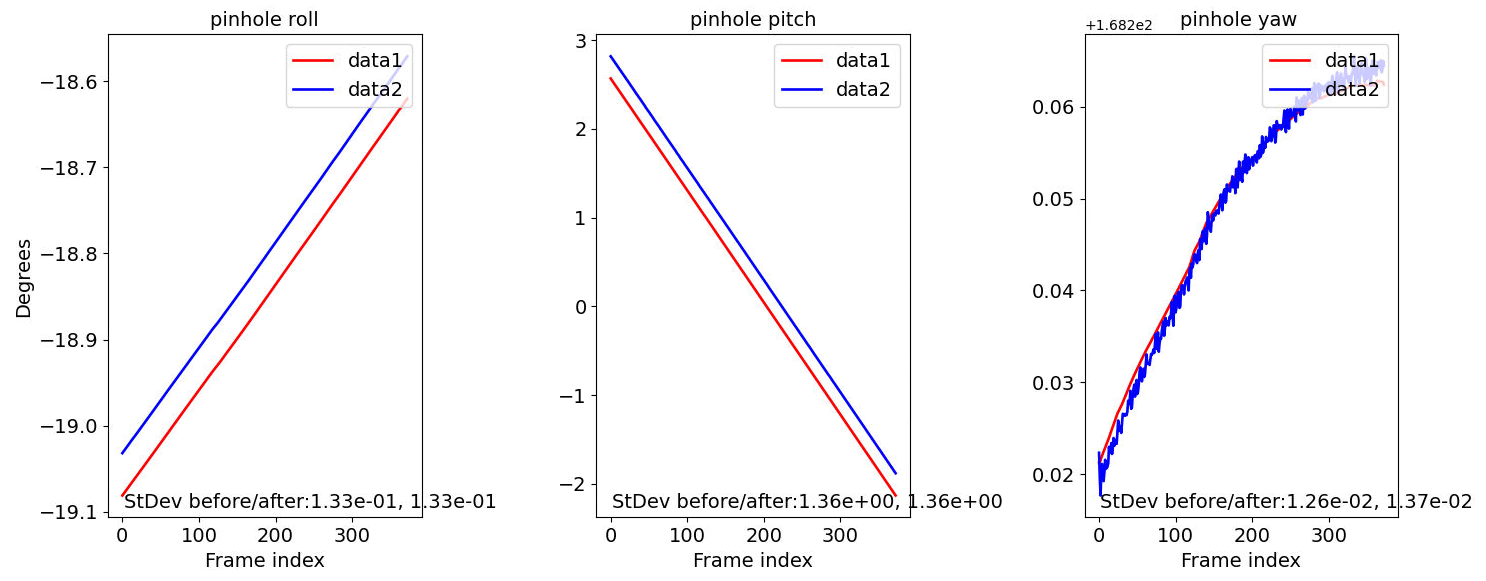
orbit_plot_fig — Fig. 16.17 Roll, pitch, and yaw angle (in degrees) for two orbital sequences, shown in red and blue.¶

16.41.3.3. Plot two orbital groups, including linescan cameras¶

Here, in addition to a group of pinhole cameras looking forward, before and after bundle adjustment, we also consider a group consisting of a single linescan camera, which looks down, before and after solving for jitter.

It is assumed that the linescan camera will have many position and orientation samples, and that these numbers of samples are equal (unless the option --use-ref-cams is used).

The only change in the command above is that the orbit id now has the additional value linescan-nadir, so the plot command becomes:

~/miniconda3/envs/orbit_plot/bin/python         \
  $(which orbit_plot.py)                        \
  --dataset dataset1/,dataset2/run-             \
  --orbit-id pinhole-fwd,linescan-nadir         \
  --dataset-label data1,data2

The cameras before optimization will be in directory dataset1/, with the pinhole camera names starting with pinhole-fwd, and the linescan camera name starting with linescan-nadir.

The cameras after optimization will start with dataset2/run-, followed again by the orbit id.

The resulting plot will have two rows, showing the two orbital groups.

16.41.4. Dependencies¶

This tool needs Python 3 and some additional Python packages to be installed with conda.

Conda can be obtained from

https://docs.conda.io/en/latest/miniconda.html

Run:

./Miniconda3-latest-Linux-x86_64.sh

on Linux, and the appropriate version on OSX (this script needs to be made executable first). Use the suggested:

$HOME/miniconda3

directory for installation.

Activate conda. The needed packages can be installed, for example, as follows:

conda create -n orbit_plot numpy scipy pyproj matplotlib

16.41.5. See also¶

The tool sfm_view (Section 16.60) can be used to visualize cameras in orbit.

16.41.6. Command-line options¶

--dataset <string (default: “”)>: The dataset to plot. If more than one, separate them by comma, with no spaces in between. The dataset is the prefix of the cameras, such as “cameras/” or “opt/run-”. It is to be followed by the orbit id, such as, “nadir” or “aft”. If more than one dataset, they will be plotted on top of each other.
--orbit-id <string (default: “”)>: The id (a string) that determines an orbital group of cameras. If more than one, separate them by comma, with no spaces in between.
--dataset-label <string (default: “”)>: The label to use for each dataset in the legend. If more than one, separate them by comma, with no spaces in between. If not set, will use the dataset name.
--orbit-label <string (default: “”)>: The label to use for each orbital group (will be shown as part of the title). If more than one, separate them by comma, with no spaces in between. If not set, will use the orbit id.
--num-cameras <int (default: -1)>: Plot only the first this many cameras from each orbital sequence. By default, plot all of them.
--use-ref-cams: Read from disk reference cameras that determine the satellite orientation. This assumes the first dataset was created with sat_sim with the option --save-ref-cams. Otherwise do not use this option. In that case the satellite orientation is estimated based on camera positions.
--subtract-line-fit: If set, subtract the best line fit from the curves being plotted.
--trim-ratio <float (default: 0.0)>: Trim ratio. Given a value between 0 and 1 (inclusive), remove this fraction of camera poses from each sequence, with half of this amount for poses at the beginning and half at the end of the sequence. This is used only for linescan cameras, to not plot camera poses beyond image lines. For cameras created with sat_sim, a value of 0.5 should be used.
--figure-size <string (default: “15,15”)>: Specify the width and height of the figure having the plots, in inches. Use two numbers with comma as separator (no spaces).
--title <string (default: “”)>: Set this as the figure title, to be shown on top of all plots.
--line-width <float (default: 1.5)>: Line width for the plots.
--font-size <int (default: 14)>: Font size for the plots.
-h, --help: Display this help message.