16.3. bathy_plane_calc¶

The bathy_plane_calc program estimates the surface of a body of water as a plane in a local stereographic projection. This plane can be slightly non-horizontal due to imperfections in the positions and orientations of the cameras that were used to create the input DEM.

Further context is given in Section 8.32.

The examples below show the several ways in which the inputs can be specified.

16.3.1. Using a camera, a mask, and a DEM¶

16.3.1.1. Preparation and running the program¶

Given a multispectral stereo dataset, a DEM obtained from a pair of images for one of the bands, a camera file from that pair, and a mask for the corresponding raw camera image delineating water from land, the water plane can be found as follows:

bathy_plane_calc --session-type dg --mask mask.tif      \
  --camera camera.xml --dem dem.tif --num-samples 10000 \
  --outlier-threshold 0.5 --bathy-plane plane.txt       \
  --output-inlier-shapefile inliers.shp

Such a mask can be obtained by thresholding an image where the water shows up darker than the land. A good example for this is the band 7 of Digital Globe multispectral images. The thresholding happens as follows:

thresh=155
image_calc -c "gt(var_0, $thresh, 1, 0)" image.tif -o mask.tif

The mask has values of 1 for land and 0 for water.

The image must be raw, not projected, and if the image is part of a stereo pair, the corresponding camera for that image must be used. In particular, if the image is multispectral, the camera must be for this dataset, not for the PAN one.

For the DEM, it is suggested to use the one obtained from PAN images, as it is more accurate, or otherwise from the Green band images. The NIR1 band is good for finding the masks, as the water is dark in them, but the DEM with NIR1 images may not be that accurate to use in this context.

It is important to decide carefully what outlier threshold to use and to check the number of resulting inliers. If too few, that may mean that the outlier threshold is too strict. Above, the inliers are saved as a shapefile and can be inspected. The inliers should be well-distributed over the entire shoreline.

For some datasets an outlier threshold of 1.0 works better than 0.5.

For a stereo pair, this tool can be run with both the left image and left camera, then separately for the right image and right camera. Ideally the results should be very similar.

The --session-type option determines which camera model to use (Digital Globe files have both an exact dg model and an approximate rpc model).

See the next section for when it is possible to use the PAN DEM and/or data with alignments applied to them.

Running this command will produce an output as follows:

Found 5017 / 13490 inliers.
Max distance to the plane (meters): 6.00301
Max inlier distance to the plane (meters): 0.499632
Mean water-surface height above datum (meters): -22.2469
Writing: plane.txt

The output file format is described in Section 16.3.10.

16.3.1.2. Handling adjusted cameras and alignment¶

The DEM and camera to be passed to bathy_plane_calc must be in the same coordinate system.

That is the case, for example, for Digital Globe images, when no bundle adjustment or alignment is performed by the user. Without these, given a stereo pair having multispectral and PAN images, the DEM obtained with the multispectral images and cameras themselves are consistent with the DEM obtained from the PAN images and corresponding cameras, with the only difference being that the multispectral images are coarser by a factor of 4, hence the resulting DEM is less precise. Therefore, it is possible to use the PAN DEM instead of multispectral DEM with this tool, while still using the multispectral cameras.

Great care must be used if bundle adjustment or alignment takes place, to keep all datasets consistent. If the multispectral images were bundle-adjusted, the same adjustments can be used with all multispectral bands. If the DEM above is obtained with bundle-adjusted multispectral images, then --bundle-adjust-prefix must be passed to bathy_plane_calc above.

If it is desired to use the PAN DEM with bathy_plane_calc, but bundle adjustment or alignment happened, with one or both of the multispectral and PAN pairs, the produced multispectral and PAN DEMs will no longer be aligned to each other. Thus, these must be individually aligned to a chosen reference DEM, the alignments applied to the cameras, as discussed in Section 16.53.14, and then the updated multispectral camera adjustments must be passed to bathy_plane_calc via --bundle-adjust-prefix.

16.3.2. Using a DEM and an orthoimage mask¶

In this example we assume that there exists a DEM and an orthoimage which is consistent with the DEM and has zero or nodata values on water and positive values on land. The bathy plane is found as follows:

bathy_plane_calc                       \
  --ortho-mask ortho_mask.tif          \
  --dem dem.tif                        \
  --outlier-threshold 0.5              \
  --bathy-plane plane.txt              \
  --output-inlier-shapefile inliers.shp

An input mask can be created, for example, with image_calc (Section 16.33.1.3). The orthoimage itself, before masking, can be produced with mapproject (Section 16.41).

16.3.3. Using a DEM and shapefile¶

This example uses a DEM and a shapefile whose vertices sample the water edge as inputs:

bathy_plane_calc                        \
  --shapefile shape.shp                 \
  --dem dem.tif                         \
  --outlier-threshold 0.5               \
  --output-inlier-shapefile inliers.shp \
  --bathy-plane plane.txt

As earlier, it is important to consider carefully what outlier threshold to use, and to examine the number and distribution of inliers.

Here it is suggested that the DEM be obtained as in the previous example, from a stereo pair, and the shapefile delineating the water-land interface be drawn on top of an orthoimage created with the same stereo pair. The commands for that can be as follows:

parallel_stereo -t dg        \
   left.tif right.tif        \
   left.xml right.xml        \
  run/run
point2dem --auto-proj-center \
  --orthoimage run/run-L.tif \
  run/run-PC.tif

See Section 6 for a discussion about various speed-vs-quality choices in stereo, and the point2dem documentation in Section 16.56.

Here is an example of a shapefile created on top of an orthoimage:

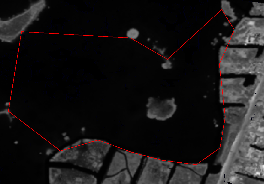
../_images/water_outline.png — Fig. 16.1 Example of a shapefile whose vertices are at the water-land boundary.¶

16.3.4. Using a DEM and lon-lat values¶

This example is similar to the one using a shapefile, but the points at which the DEM is sampled are provided in a CSV file having longitude and latitude values:

bathy_plane_calc                        \
  --lon-lat-measurements meas.csv       \
  --csv-format "2:lon 3:lat"            \
  --dem dem.tif                         \
  --outlier-threshold 0.5               \
  --output-inlier-shapefile inliers.shp \
  --bathy-plane plane.txt

The heights will be looked up in the DEM with bilinear interpolation. The longitude and latitude will be interpreted relative to the DEM georeference.

The --csv-format option must be set correctly to identify the columns having the longitude and latitude. The CSV file can have other columns as well (such as an ID), which will be ignored. See Section 16.3.6 for more details on the CSV format.

16.3.5. Using a water-surface raster¶

Given a water-surface raster (Section 16.3.10.2), this mode writes its best-fit plane in plain-text format (Section 16.3.10.1). The plane is fit in a local stereographic projection:

bathy_plane_calc                    \
  --water-surface water_surface.tif \
  --bathy-plane plane.txt

This is for inspecting or comparing the plane against the raster surface (Section 16.9.1.7). The parallel_stereo program accepts the water surface raster directly (Section 8.32.6).

16.3.6. Using water height measurements¶

In this example, a set of actual measurements of the water surface is provided, as the longitude and latitude (in degrees, in decimal format), and water height above the WGS_1984 datum (ellipsoid heights), measured in meters.

If the water heights are given relative to a geoid (such as EGM2008), or some other datum (such as NAD83), those need to be converted to WGS_1984.

It is expected that the measurements are given in a CSV file, with commas or spaces used as separators. A procedure for collecting such data is outlined further down this document (Section 16.3.8). Here is an sample file, named meas.csv, for Florida Keys:

FID,Lon,Lat,WGS84_m
0,-81.59864018,24.58775288,-23.86539
1,-81.62377319,24.58180388,-23.84653
2,-81.62987019,24.57838388,-23.8864
3,-81.6745502,24.56443387,-23.86815
4,-81.71131321,24.55574886,-23.86031
5,-81.75447022,24.55158486,-23.85464
6,-81.75601722,24.55176286,-23.89892
7,-81.77999023,24.54843186,-23.89824

Any lines starting with the pound sign (#) will be ignored as comments. If the first line does not start this way but does not have valid data it will be ignored as well. Empty lines will be ignored too.

The program is called as follows:

bathy_plane_calc --water-height-measurements meas.csv  \
  --csv-format "2:lon 3:lat 4:height_above_datum"      \
  --outlier-threshold 0.5 --bathy-plane meas_plane.txt \
  --output-inlier-shapefile meas_inliers.shp

Note the --csv-format option, which should be set correctly. As specified here, it will result in columns 2, 3, and 4, being read, having the longitude, latitude, and height above datum (WGS84 ellipsoid). The order in which the columns show up is not important, as long as --csv-format correctly reflects that. Any extraneous columns will be ignored, such as the ID in column 1.

Care must be taken to ensure all the measurements, resulting bathy plane, and any DEMs are in the same coordinate system. This is discussed further in Section 8.32.8.

16.3.7. Pick a sample set of points at the water-land boundary¶

In this example, instead of computing the best-fitting plane, bathy_plane_calc finds a set of samples (given by --num-samples) at the water-land interface and saves them as a shapefile of points, having longitude-latitude pairs relative to the WGS_1984 datum (ellipsoid).

Example:

bathy_plane_calc --session-type dg --mask mask.tif    \
  --camera camera.xml --dem dem.tif --num-samples 100 \
  --mask-boundary-shapefile samples.shp

When the input is a mask, a random sample is picked (their number given by --num-samples). The heights are looked up in the DEM if not already present in the input.

This shapefile may then be passed to some external tool for looking up water level heights at these points.

16.3.8. Acquisition of water height data¶

This section describes how to acquire a set of water height measurements, which then could be used to create the best-fit water plane for the purpose of shallow-water bathymetry. An example of using this data is given in Section 16.3.6.

Absent direct measurements of water surface level at the date and time of satellite image acquisition, it is suggested to use the discrete tidal zoning information provided by the National Ocean Service , while for the metadata use the CO-OPS Discrete Tidal Zoning Map. An organizational Esri GIS online login is needed to access the data.

Each polygon on the map is a discrete tidal zone, within which NOAA considers the tide characteristics the same. If the user clicks a polygon on the map, a window will pop up and show the control tide station (ControlStn) for that zone, average time corrector (AvgTimeCorr, in minutes), and range ratio (RangeRatio). Note that:

The control station is usually an active water level station of NOAA.

Average time corrector is the time difference (phase difference) between the tide at the tide zone and at the control station. Positive time means the tide level is this many minutes later in the tidal zone polygon than at the control station (and vice versa).

Range ratio is the ratio of tide range at the tidal zone divided by that at the control station.

The user can access tidal gauge data for the satellite day and time of acquisition at the Center for Operational Oceanographic Products and Services. Choose Verified Data-> Six Minutes Data->Try me.

The user can download tide data in any reference as long as the value is expressed in meters. This value needs to be transformed into an ellipsoid heights value relative to the WGS_1984 datum. For this the NOAA VDATUM Java program can be used, or the NOAA online app.

Please note that even if lots of points on the land/water limit belong to the same tidal zone polygon, so they will have same elevation value, the transformation in ellipsoid heights with VDATUM will result in different ellipsoid heights since VDATUM uses the position of the point in latitude/longitude besides the height of the point.

Export your data to a CSV file with a header containing ID, longitude, latitude, and WGS_1984 height measurements.

16.3.9. Global tide models and water surface elevation¶

The ASP bathymetry module requires a water surface elevation plane corresponding to the date and time of satellite image acquisition. This input may be provided either as a text file containing water plane model parameters (Section 16.3.10.1) or as a water surface elevation raster (Section 16.3.10.2). The georeferenced water surface raster is commonly sourced externally by combining the global mean sea surface with the appropriate global tide raster model, matched to the relevant date and time for the processed satellite images.

Typically, the global tide model expresses water surface elevations in meters (or centimeters) above mean sea surface (MSS), referenced to the Earth’s ellipsoid based on satellite altimetry, or above mean sea level (MSL) derived from tide-gauge measurements, and aligned to land-based vertical datums (usually orthometric). Several global tide services are available, including:

AVISO FES22 (Finite Element Solution), which leverages finite-element hydrodynamics, altimeter and tide-gauge measurements, and loading data, accessed through the Archiving, Validation and Interpretation of Satellite Oceanographic (AVISO+) portal.
TPXO10 / OTIS (Tidal Prediction eXpanded and Ocean Tides Inversion System), a global and regional barotropic tide modeling system developed by Oregon State University.
NASA Goddard Ocean Tide (GOT) series, providing empirical fits derived from altimeter data for both short-period (diurnal/semidiurnal) and long-period tides.
DTU10 global ocean tide model from the Technical University of Denmark, based on multi-mission satellite altimetry extending into coastal regions.
EOT20, the global empirical ocean tide model developed by the German Geodetic Research Institute, Technical University of Munich (DGFI-TUM), utilizing multi-mission altimetry data.

The resultant water surface elevation raster is computed by adding MSS (or MSL converted to ellipsoid heights) and the tide values extracted for the satellite image area of interest, at their exact acquisition date and time.

The ASP bathymetry module underwent extensive validation using water surface elevations derived from AVISO+ MSS and extrapolated FES22 data for geocentric tides. The FES22 geocentric tide model consists of two elements: (a) ocean tide extrapolated into coastal and shallow waters, illustrating vertical displacement due to tidal forces relative to the ocean floor, and (b) tidal loading, reflecting Earth’s elastic response to ocean water redistribution during tidal events.

16.3.10. Bathy plane definition and format¶

The bathy plane represents the surface of the water at the time of image acquisition. It can have one of two formats: a plain-text file with four plane coefficients in local projected coordinates, or a georeferenced raster of water-surface heights (in either a projected or a geographic CRS).

The plain-text format is produced by bathy_plane_calc. The georeferenced-raster format is typically an external water-surface product (e.g., the mean sea surface plus tide at image acquisition time).

16.3.10.1. Plain text bathy plane¶

In this mode, the bathy plane ends with a .txt extension. It will look like this:

-0.0090 0.0130 0.9998 22.2460
# Latitude and longitude of the local stereographic projection with the WGS_1984 datum:
24.5836 -81.7730

The last line has the center of the local stereographic projection in which the plane is computed, and the first line has the equation of the plane in that local coordinate system as:

a * x + b * y + c * z + d = 0.

The value of c is almost 1, hence this plane is almost perfectly horizontal in local coordinates and the value of -d/c gives its height above the datum (The small deviation from the horizontal may be due to the orientations of the satellites taking the pictures not being perfectly known.)

16.3.10.2. Georeferenced raster bathy plane¶

Alternatively, the bathy plane can be provided as a georeferenced raster of per-pixel water-surface heights above the WGS_1984 ellipsoid, in meters, with an optional no-data value. In this mode, the file is formatted like a DEM. The projection can be either geographic (lon-lat) or in meters.

The pixel values must be ellipsoid heights, rather than orthometric heights or heights above a geoid.

A typical source is the mean sea surface (e.g. MSS_CNES_CLS2022) plus the geocentric tide at image acquisition time (e.g. from FES2022b).

See Section 16.3.5 for how to convert a bathy plane in raster format to the plain-text format.

See Section 16.9.1.7 for how to quickly test such a bathy plane (in either format), or for comparing the same surface specified in different formats.

See Section 16.3.9 for global tide models and how to combine them with mean sea surface to produce a water surface elevation raster.

16.3.11. Command-line options for bathy_plane_calc¶

--shapefile <filename>: The shapefile with vertices whose coordinates will be looked up in the DEM with bilinear interpolation.
--dem <filename>: The DEM to use.
--mask <string (default: “”)>: An input mask, created from a raw camera image and hence having the same dimensions, with values of 1 on land and 0 on water, or positive values on land and nodata values on water. The larger of the nodata value and zero is used as the water value. The heights will be looked up in the DEM with bilinear interpolation.
--camera <string (default: “”)>: The camera file to use with the mask.
--bathy-plane arg: The output file storing the computed plane (Section 16.3.10).
--output-inlier-shapefile <string (default: “”)>: If specified, save at this location the shape file with the inlier vertices.
--output-outlier-shapefile <string (default: “”)>: If specified, save at this location the shape file with the outlier vertices.
--bundle-adjust-prefix <string (default: “”)>: Use the camera adjustment at this output prefix, if the cameras changed based on bundle adjustment or alignment.
-t, --session-type <string (default: “”)>: Select the stereo session type to use for processing. Usually the program can select this automatically by the file extension, except for xml cameras. See Section 16.51.8 for options.
--outlier-threshold <double>: A value, in meters, to determine the distance from a sampled point on the DEM to the best-fit plane to determine if it will be marked as outlier and not included in the calculation of that plane. The default is 0.5. Its value should be roughly the expected vertical uncertainty of the DEM.
--num-ransac-iterations <integer>: Number of RANSAC iterations to use to find the best-fitting plane. The default is 1000.
--num-samples <integer>: Number of samples to pick at the water-land interface if using a mask. The default is 10000.
--ortho-mask <filename>: An input mask, that is georeferenced and aligned with the DEM, with positive values on land and 0 or nodata values on water. The larger of the nodata value and zero is used as the water value.
--lon-lat-measurements <string (default: “”)>: Use this CSV file having longitude and latitude measurements for the water surface. The heights will be looked up in the DEM with bilinear interpolation. The option –csv-format must be used.
--water-height-measurements <string (default: “”)>: Use this CSV file having longitude, latitude, and height measurements for the water surface, in degrees and meters, respectively, relative to the WGS84 datum. The option –csv-format must be used.
--csv-format <string (default: “”)>: Specify the format of the CSV file having water height measurements or longitude and latitude values. The format should have a list of entries with syntax column_index:column_type (indices start from 1). Example: ‘2:lon 3:lat 4:height_above_datum’. Note that this option must be enclosed in quotes so it is parsed correctly by the shell. See Section 19.12 for details.
--mask-boundary-shapefile <string (default: “”)>: If specified, save the extracted points (before RANSAC) to this shapefile and exit. When the input is a mask, a random sample is picked (their number given by --num-samples). The heights are looked up in the DEM if not already present in the input. See an example in Section 16.3.7.
--save-shapefiles-as-polygons: Save the inlier and outlier shapefiles as polygons, rather than made of discrete vertices. May be more convenient for processing in a GIS tool.
--dem-minus-plane <string (default: “”)>: If specified, subtract from the input DEM the best-fit plane and save the obtained DEM to this GeoTiff file.
--water-surface <string (default: “”)>: Takes as input a georeferenced raster of per-pixel water-surface heights above the WGS_1984 ellipsoid, in meters, with an optional no-data value (see Section 16.3.10.2). The best-fit plane to this raster is computed in a local stereographic projection and written to --bathy-plane for inspection or comparison. No DEM, mask, shapefile, or measurement file is required in this mode (see Section 16.3.5).
--threads <integer (default: 0)>: Select the number of threads to use for each process. If 0, use the value in ~/.vwrc.
--cache-size-mb <integer (default = 1024)>: Set the system cache size, in MB.
--tile-size <integer (default: 256 256)>: Image tile size used for multi-threaded processing.
--no-bigtiff: Tell GDAL to not create BigTiff files.
--tif-compress <None|LZW|Deflate|Packbits (default: LZW)>: TIFF compression method.
-v, --version: Display the version of software.
-h, --help: Display this help message.