12. Bundle adjustment
12.1. Overview
Satellite position and orientation errors have a direct effect on the accuracy of digital elevation models produced by the Stereo Pipeline. If they are not corrected, these uncertainties will result in systematic errors in the overall position and slope of the DEM. Severe distortions can occur as well, resulting in twisted or “taco-shaped” DEMs, though in most cases these effects are quite subtle and hard to detect. In the worst case, such as with old mission data like Voyager or Apollo, these gross camera misalignments can inhibit Stereo Pipeline’s internal interest point matcher and block auto search range detection.
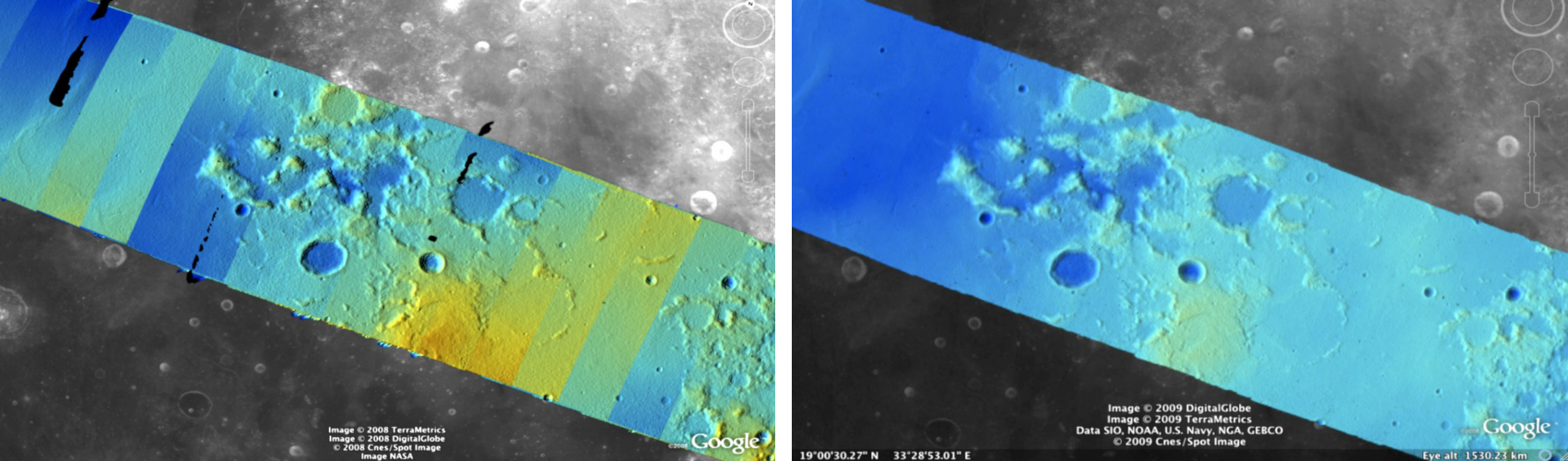
Fig. 12.1 Bundle adjustment is illustrated here using a color-mapped, hill-shaded DEM mosaic from Apollo 15, Orbit 33, images. (a) Prior to bundle adjustment, large discontinuities can exist between overlapping DEMs made from different images. (b) After bundle adjustment, DEM alignment errors are minimized and no longer visible.
Errors in camera position and orientation can be corrected using a process called bundle adjustment. Bundle adjustment is the process of simultaneously adjusting the properties of many cameras and the 3D locations of the objects they see in order to minimize the error between the estimated, back-projected pixel locations of the 3D objects and their actual measured locations in the captured images. This is called the reprojection error.
This complex process can be boiled down to this simple idea: bundle adjustment ensures that the observations in multiple images of a single ground feature are self-consistent. If they are not consistent, then the position and orientation of the cameras as well as the 3D position of the feature must be adjusted until they are. This optimization is carried out along with thousands (or more) of similar constraints involving many different features observed in other images. Bundle adjustment is very powerful and versatile: it can operate on just two overlapping images, or on thousands. It is also a dangerous tool. Careful consideration is required to insure and verify that the solution does represent reality.
Bundle adjustment can also take advantage of GCPs (Section 16.5.9), which are
3D locations of features that are known a priori (often by measuring them by
hand in another existing DEM). GCPs can improve the internal consistency of your
DEM or align your DEM to an existing data product. Finally, even though bundle
adjustment calculates the locations of the 3D objects it views, only the final
properties of the cameras are recorded for use by the Ames Stereo Pipeline.
Those properties can be loaded into the parallel_stereo program which uses
its own method for triangulating 3D feature locations.
When using the Stereo Pipeline, bundle adjustment is an optional step
between the capture of images and the creation of DEMs. The bundle
adjustment process described below should be completed prior to running
the parallel_stereo command.
Although bundle adjustment is not a required step for generating DEMs, it is highly recommended for users who plan to create DEMs for scientific analysis and publication. Incorporating bundle adjustment into the stereo work flow not only results in DEMs that are more internally consistent, it is also the correct way to co-register your DEMs with other existing data sets and geodetic control networks.
A DEM obtained after bundle adjustment and stereo may need to be aligned
to a known reference coordinate system. For that, use the pc_align
tool (Section 16.53).
See the options --heights-from-dem (Section 12.2.1.3)
and --reference-terrain further down for how to incorporate an
external DEM in bundle adjustment. Note that these can only locally
refine camera parameters, an initial alignment with pc_align is
still necessary.
Optimizing of camera intrinsics parameters, such as optical center, focal length, and distortion is also possible, as seen below.
12.2. Running bundle adjustment
Stereo Pipeline provides the bundle_adjust program
(Section 16.5).
Start by running parallel_stereo without using bundle-adjusted camera
models:
parallel_stereo AS15-M-1134.cub AS15-M-1135.cub run_noadjust/run
See Section 6 for how how to improve the quality of stereo correlation results (at the expense of speed).
Create a DEM and triangulation error image as in Section 16.56.
Run bundle adjustment:
bundle_adjust --camera-position-weight 0     \
 --tri-weight 0.1 --tri-robust-threshold 0.1 \
 AS15-M-1134.cub AS15-M-1135.cub -o run_ba/run
Here only camera positions and orientations are refined. How to optimize the camera intrinsics (if applicable) is discussed further down (Section 12.2.1).
Run parallel_stereo while using the bundle-adjusted camera models:
parallel_stereo AS15-M-1134.cub AS15-M-1135.cub \
  --prev-run-prefix run_noadjust/run            \
  --bundle-adjust-prefix run_ba/run             \
  run_adjust/run
This should be followed, as before, by creation of a DEM and a triangulation
error image. Note the option --prev-run-prefix that allowed reusing
the previous run apart from the triangulation step. That speeds up the process,
and works well-enough unless the cameras change a lot.
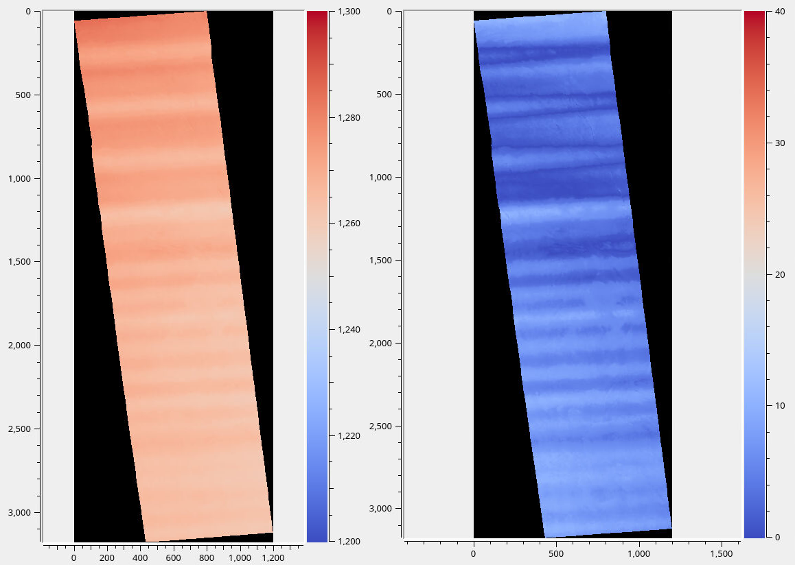
Fig. 12.2 An unusually large intersection error (left), and the version after bundle adjustment (right). Note that these do not use the same range of colors. The images are produced with the MOC camera (Section 8.4). The remaining wavy pattern is due to jitter, that ASP has a solver for (Section 16.38). More illustrations are in Section 12.2.5 and Section 12.2.3.5.
Bundle adjustment aims to make the cameras more self-consistent but offers no
guarantees about their absolute positions (unless GCP are used,
Section 16.5.9), in fact, the cameras can move away a lot sometimes. The
options --tri-weight, --rotation-weight, and
--camera-position-weight can be used to constrain how much the cameras can
move during bundle adjustment. Note that large values for these may impact the
ability to make the cameras self-consistent.
This program can constrain the triangulated points, and hence the cameras, relative to a DEM. This option only works when the cameras are already rather well-aligned to this DEM and only fine-level adjustments are needed. That is discussed in Section 12.2.1.3.
ASP also offers the tool parallel_bundle_adjust which can create
match files using multiple processes spread over multiple machines
(Section 16.49). These can also be used later
during stereo with the options --match-files-prefix and
--clean-match-files-prefix.
12.2.1. Floating intrinsics and using a lidar or DEM ground truth
This section documents some advanced functionality, and it suggested the reader study it carefully and invest a certain amount of time to fully take advantage of these concepts.
When the input cameras are of Pinhole type (Section 20.1), optical bar (Section 20.2), or CSM (Section 8.12), it is possible to optimize (float, refine) the intrinsic parameters (focal length, optical center, distortion, with a somewhat different list for optical bar cameras), in addition to the extrinsics.
It is also possible to take advantage of an existing terrain ground truth, such as a lidar file or a DEM, to correct imperfectly calibrated intrinsic parameters, which can result in greatly improved results, such as creating less distorted DEMs that agree much better with the ground truth.
See Section 12.2.1.1 for how to optimize intrinsics with no constraints, Section 12.2.1.2 for when ground constraints can be used (there exist options for sparse ground points and a DEM), and Section 12.2.2 for how to have several groups of intrinsics.
Mixing frame and linescan cameras is discussed in Section 12.2.3.
12.2.1.1. A first attempt at floating the intrinsics
This section is only an introduction of how to float the intrinsics. Detailed examples are further down.
It is very strongly suggested to ensure that a good number of images exists, they have a lot of overlap, that the cameras have been already bundle-adjusted with intrinsics fixed and aligned to a DEM (Section 16.53.14). Such a DEM should be used as a constraint.
Note that when solving for intrinsics, bundle_adjust will by default
optimize all intrinsic parameters and will share them across all cameras. This
behavior can be controlled with the --intrinsics-to-float and
--intrinsics-to-share parameters, or in a finer-grained way, as shown in
Section 12.2.2.
The first invocation of camera optimization should be with intrinsics fixed:
bundle_adjust -t nadirpinhole --inline-adjustments      \
  left.tif right.tif left.tsai right.tsai -o run_ba/run
Here two images have been used for illustration purposes, but a larger number should be used in practice.
It is suggested that one run parallel_stereo with the obtained cameras:
parallel_stereo -t nadirpinhole --alignment-method epipolar      \
   --stereo-algorithm asp_mgm --subpixel-mode 9                  \
   left.tif right.tif run_ba/run-left.tsai run_ba/run-right.tsai \
   run_stereo/run
followed by DEM creation (Section 16.56):
point2dem --tr RESOLUTION --errorimage run_stereo/run-PC.tif
Then examine and plot the intersection error:
gdalinfo -stats run_stereo/run-IntersectionErr.tif
colormap run_stereo/run-IntersectionErr.tif
stereo_gui run_stereo/run-IntersectionErr_CMAP.tif
See Section 6.1 for other stereo algorithms. For colormap
(Section 16.14), --min and --max bounds can be specified if the
automatic range is too large.
We also suggest inspecting the interest points (Section 16.71.9):
stereo_gui left.tif right.tif run_ba/run
and then viewing the interest points from the menu.
If the interest points are not well-distributed, this may result in large ray intersection errors where they are missing. Then, one should delete the existing run directory and create a better set, as discussed in Section 12.2.4.
If the interest points are good and the mean intersection error is acceptable, but this error shows an odd nonlinear pattern, that means it may be necessary to optimize the intrinsics. We do so by using the cameras with the optimized extrinsics found earlier. This is just an early such attempt, better approaches will be suggested below:
bundle_adjust -t nadirpinhole --inline-adjustments \
  --solve-intrinsics --camera-position-weight 0    \
  --max-pairwise-matches 20000                     \
  left.tif right.tif                               \
  run_ba/run-left.tsai run_ba/run-right.tsai       \
  -o run_ba_intr/run
See Section 12.2.1.3 for how to use a DEM as a constraint. See Section 12.2.4.2 for how to create dense interest points. Both of these are very recommended.
It is important to note that only the non-zero intrinsics will be optimized, and the step size used in optimizing a certain intrinsic parameter is proportional to it. Hence, if an intrinsic is 0 and it is desired to optimize it, it should be set to small non-zero value suggestive of its final estimated scale. If the algorithm fails to give a good solution, perhaps different initial values for the intrinsics should be tried. For example, one can try changing the sign of the initial distortion coefficients, or make their values much smaller.
It is good to use a lens distortion model such as the one ASP calls Tsai (Section 20.1), as then the distortion operation is a simple formula, which is fast and convenient in bundle adjustment, when projecting into the camera is the key operation. Using models like Photometrix and Brown-Conrady is not advised.
Here we assumed all intrinsics are shared. See
Section 12.2.2 for how to have several groups of
intrinsics. See also the option --intrinsics-to-share.
Sometimes the camera weight may need to be decreased, even all the way to 0, if it appears that the solver is not aggressive enough, or it may need to be increased if perhaps it overfits. This will become less of a concern if there is some ground truth, as discussed later.
Next, one can run parallel_stereo as before, with the new cameras, and see
if the obtained solution is more acceptable, that is, if the intersection error
is smaller. It is good to note that a preliminary investigation can already be
made right after bundle adjustment, by looking at the residual error files
before and after bundle adjustment. They are in the bundle_adjust output
directory, with names:
initial_residuals_pointmap.csv
final_residuals_pointmap.csv
If desired, these csv files can be converted to a DEM with
point2dem, which can be invoked with:
--csv-format 1:lon,2:lat,4:height_above_datum
then one can look at their statistics, also have them colorized, and
viewed in stereo_gui (Section 16.71.6).
This file also shows how often each feature is seen in the images, so, if three images are present, hopefully many features will be seen three times.
12.2.1.2. Using ground truth when floating the intrinsics
If a point cloud having ground truth, such as a DEM or lidar file
exists, say named ref.tif, it can be used as part of bundle
adjustment. For that, the stereo DEM obtained earlier
needs to be first aligned to this ground truth, such as:
pc_align --max-displacement VAL           \
  run_stereo/run-DEM.tif ref.tif          \
  --save-inv-transformed-reference-points \
  -o run_align/run
(see the manual page of this tool in Section 16.53 for more details).
This alignment can then be applied to the cameras as well:
bundle_adjust -t nadirpinhole --inline-adjustments              \
  --initial-transform run_align/run-inverse-transform.txt       \
  left.tif right.tif run_ba/run-left.tsai run_ba/run-right.tsai \
  --apply-initial-transform-only -o run_align/run
If pc_align is called with the clouds in reverse order (the denser
cloud should always be the first), when applying the transform to the
cameras in bundle_adjust one should use transform.txt instead of
inverse-transform.txt above.
Note that if your ground truth is in CSV format, any tools that use this cloud
must set --csv-format and perhaps also --datum and/or --csv-srs.
See Section 16.53.14 for how to handle the case when input adjustments exist.
There are two ways of incorporating a ground constraint in bundle adjustment. The first one assumes that the ground truth is a DEM, and is very easy to use with a large number of images (Section 12.2.1.3). A second approach can be used when the ground truth is sparse (and with a DEM as well). This is a bit more involved (Section 12.2.1.4).
12.2.1.3. Using the heights from a reference DEM
In some situations the DEM obtained with ASP is, after alignment, quite similar to a reference DEM, but the heights may be off. This can happen, for example, if the focal length or lens distortion are not accurately known.
In this case it is possible to borrow more accurate information from the
reference DEM. The option for this is --heights-from-dem. An additional
control is given, in the form of the option --heights-from-dem-uncertainty
(1 sigma, in meters). The smaller its value is, the stronger the DEM constraint.
This value divides the difference between the triangulated points being
optimized and their initial value on the DEM when added to the cost function
(Section 16.5.8).
The option --heights-from-dem-robust-threshold ensures that these weighted
differences plateau at a certain level and do not dominate the problem. The
default value is 0.1, which is smaller than the --robust-threshold value of
0.5, which is used to control the pixel reprojection error, as that is given a
higher priority. It is suggested to not modify this threshold, and adjust
instead --heights-from-dem-uncertainty.
If a triangulated point is not close to the reference DEM, bundle adjustment
falls back to the --tri-weight constraint.
Here is an example when we solve for intrinsics with a DEM constraint. As in the earlier section, we assume that the cameras and the terrain are already aligned:
bundle_adjust -t nadirpinhole               \
  --inline-adjustments                      \
  --solve-intrinsics                        \
  --intrinsics-to-float all                 \
  --intrinsics-to-share all                 \
  --camera-position-weight 0                \
  --max-pairwise-matches 20000              \
  --heights-from-dem dem.tif                \
  --heights-from-dem-uncertainty 10.0       \
  --parameter-tolerance 1e-12               \
  --remove-outliers-params "75.0 3.0 20 25" \
  left.tif right.tif                        \
  run_align/run-run-left.tsai               \
  run_align/run-run-right.tsai              \
  -o run_ba_hts_from_dem/run
One should be careful with setting --heights-from-dem-uncertainty. Having
it larger will ensure it does not prevent convergence.
It is strongly suggested to use dense interest points (Section 12.2.4.2), if
solving for intrinsics, and have --max-pairwise-matches large enough to not
throw some of them out. We set --camera-position-weight 0, as hopefully the
DEM constraint is enough to constrain the solution.
Here we were rather generous with the parameters for removing outliers, as the input DEM may not be that accurate, and then if tying too much to it some valid matches be be flagged as outliers otherwise, perhaps.
The implementation of --heights-from-dem is as follows. Rays from matching
interest points are intersected with this DEM, and the average of the produced
points is projected vertically onto the DEM. This is declared to be the
intersection point of the rays, and the triangulated points being optimized
are constrained via --heights-from-dem-uncertainty to be close to this
point.
It is important to note that this heuristic may not be accurate if the rays have a large intersection error. But, since bundle adjustment usually has two passes, at the second pass the improved cameras are used to recompute the point on the DEM with better accuracy.
This option can be more effective than using --reference-terrain when there
is a large uncertainty in camera intrinsics.
See two other large-scale examples of using --heights-from-dem, without
floating the intrinsics, in the SkySat processing example (Section 8.27),
using Pinhole cameras, and with linescan Lunar images with variable illumination
(Section 11.10).
Here we assumed all intrinsics are shared. See Section 12.2.2 for how to
have several groups of intrinsics. See also the option
--intrinsics-to-share.
It is suggested to look at the documentation of all the options above and adjust them for your use case.
See Section 16.5 for the documentation of all options above, and Section 16.5.11 for the output reports being saved, which can help judge how well the optimization worked.
12.2.1.4. Sparse ground truth and using the disparity
Here we will discuss an approach that works when the ground truth can be sparse, and we make use of the stereo disparity. It requires more work to set up than the earlier one.
We will need to create a disparity from the left and right images that we will use during bundle adjustment. For that we will take the disparity obtained in stereo and remove any intermediate transforms stereo applied to the images and the disparity. This can be done as follows:
stereo_tri -t nadirpinhole --alignment-method epipolar \
  --unalign-disparity                                  \
  left.tif right.tif                                   \
  run_ba/run-left.tsai run_ba/run-right.tsai           \
  run_stereo/run
and then bundle adjustment can be invoked with this disparity and the DEM/lidar file. Note that we use the cameras obtained after alignment:
bundle_adjust -t nadirpinhole --inline-adjustments         \
  --solve-intrinsics --camera-position-weight 0            \
  --max-disp-error 50                                      \
  --max-num-reference-points 1000000                       \
  --max-pairwise-matches 20000                             \
  --parameter-tolerance 1e-12                              \
  --robust-threshold 2                                     \
  --reference-terrain lidar.csv                            \
  --reference-terrain-weight 5                             \
  --disparity-list run_stereo/run-unaligned-D.tif          \
  left.tif right.tif                                       \
  run_align/run-run-left.tsai run_align/run-run-right.tsai \
  -o run_ba_intr_lidar/run
Here we set the camera weight all the way to 0, since it is hoped that having a reference terrain is a sufficient constraint to prevent over-fitting.
We used --robust-threshold 2 to make the solver work harder
where the errors are larger. This may be increased somewhat if the
distortion is still not solved well in corners.
See the note earlier in the text about what a good lens distortion model is.
This tool will write some residual files of the form:
initial_residuals_reference_terrain.txt
final_residuals_reference_terrain.txt
which may be studied to see if the error-to-lidar decreased. Each residual is defined as the distance, in pixels, between a terrain point projected into the left camera image and then transferred onto the right image via the unaligned disparity and its direct projection into the right camera.
If the initial errors in that file are large to start with, say more than 2-3 pixels, there is a chance something is wrong. Either the cameras are not well-aligned to each other or to the ground, or the intrinsics are off too much. In that case it is possible the errors are too large for this approach to reduce them effectively.
We strongly recommend that for this process one should not rely on bundle adjustment to create interest points, but to use the dense and uniformly distributed ones created with stereo (Section 12.2.4.2).
The hope is that after these directions are followed, this will result
in a smaller intersection error and a smaller error to the lidar/DEM
ground truth (the later can be evaluated by invoking
geodiff --absolute on the ASP-created aligned DEM and the reference
lidar/DEM file).
Here we assumed all intrinsics are shared. See
Section 12.2.2 for how to have several groups of
intrinsics. See also the option --intrinsics-to-share.
When the lidar file is large, in bundle adjustment one can use the flag
--lon-lat-limit to read only a relevant portion of it. This can
speed up setting up the problem but does not affect the optimization.
12.2.1.5. Sparse ground truth and multiple images
Everything mentioned earlier works with more than two images, in fact, having more images is highly desirable, and ideally the images overlap a lot. For example, one can create stereo pairs consisting of first and second images, second and third, third and fourth, etc., invoke the above logic for each pair, that is, run stereo, alignment to the ground truth, dense interest point generation, creation of unaligned disparities, and transforming the cameras using the alignment transform matrix. Then, a directory can be made in which one can copy the dense interest point files, and run bundle adjustment with intrinsics optimization jointly for all cameras. Hence, one should use a command as follows (the example here is for 4 images):
disp1=run_stereo12/run-unaligned-D.tif
disp2=run_stereo23/run-unaligned-D.tif
disp3=run_stereo34/run-unaligned-D.tif
bundle_adjust -t nadirpinhole --inline-adjustments       \
  --solve-intrinsics  --camera-position-weight 0         \
  img1.tif img2.tif img3.tif img4.tif                    \
  run_align_12/run-img1.tsai run_align12/run-img2.tsai   \
  run_align_34/run-img3.tsai run_align34/run-img4.tsai   \
  --reference-terrain lidar.csv                          \
  --disparity-list "$disp1 $disp2 $disp3"                \
  --robust-threshold 2                                   \
  --max-disp-error 50 --max-num-reference-points 1000000 \
  --overlap-limit 1 --parameter-tolerance 1e-12          \
  --reference-terrain-weight 5                           \
  -o run_ba_intr_lidar/run
In case it is desired to omit the disparity between one pair of images,
for example, if they don’t overlap, instead of the needed unaligned
disparity one can put the word none in this list.
Notice that since this joint adjustment was initialized from several stereo pairs, the second camera picked above, for example, could have been either the second camera from the first pair, or the first camera from the second pair, so there was a choice to make. In Section 8.27 an example is shown where a preliminary bundle adjustment happens at the beginning, without using a reference terrain, then those cameras are jointly aligned to the reference terrain, and then one continues as done above, but this time one need not have dealt with individual stereo pairs.
The option --overlap-limit can be used to control which images
should be tested for interest point matches, and a good value for it is
say 1 if one plans to use the interest points generated by stereo,
though a value of 2 may not hurt either. One may want to decrease
--parameter-tolerance, for example, to 1e-12, and set a value for
--max-disp-error, e.g, 50, to exclude unreasonable disparities (this
last number may be something one should experiment with, and the results
can be somewhat sensitive to it). A larger value of
--reference-terrain-weight can improve the alignment of the cameras
to the reference terrain.
Also note the earlier comment about sharing and floating the intrinsics individually.
12.2.2. Refining the intrinsics per sensor
Given a set of sensors, with each acquiring several images, we will optimize the intrinsics per sensor. All images acquired with the same sensor will share the same intrinsics, and none will be shared across sensors.
We will work with Kaguya TC linescan cameras and the CSM camera model (Section 8.12). Pinhole cameras in .tsai format (Section 20.1) and Frame cameras in CSM format (Section 20.3) can be used as well.
See Section 12.2.1 for an introduction on how optimizing intrinsics works, and Section 8.14 for how to prepare and use Kaguya TC cameras.
See Section 12.2.3 for fine-level control per group and for how to mix frame and linescan cameras.
12.2.2.1. Things to watch for
Optimizing the intrinsics can be tricky. One has to be careful to select a non-small set of images that have a lot of overlap, similar illumination, and an overall good baseline between enough images (Section 8.1).
It is suggested to do a lot of inspections along the way. If things turn out to work poorly, it is often hard to understand at what step the process failed. Most of the time the fault lies with the data not satisfying the assumptions being made.
The process will fail if, for example, the data is not well-aligned before the refinement of intrinsics is started, if the illumination is so different that interest point matches cannot be found, or if something changed about a sensor and the same intrinsics don’t work for all images acquired with that sensor.
The cam_test tool (Section 16.9) can be used to check if the distortion
model gets inverted correctly. The distortion model should also be expressive
enough to model the distortion in the images.
12.2.2.2. Image selection
We chose a set of 10 Kaguya stereo pairs with a lot of overlap (20 images in
total). The left image was acquired with the TC1 sensor, and the right one
with TC2. These sensors have different intrinsics.
Some Kaguya images have different widths. These should not be mixed together. Of the images with narrower width, it was observed that images acquired with “morning” illumination need different calibration than the rest. Hence, there will be two groups of intrinsics for the narrow TC images.
Some images had very large difference in illumination (not for the same stereo
pair). Then, finding of matching interest points can fail. Kaguya images are
rather well-registered to start with, so the resulting small misalignment that
could not be corrected by bundle adjustment was not a problem in solving for
intrinsics, and pc_align (Section 16.53) was used later for individual
alignment. This is not preferable, in general. It was tricky however to find
many images with a lot of overlap, so this had to make do.
A modification of the work flow for the case of images with very different illumination is in Section 12.2.2.10.
12.2.2.3. Initial bundle adjustment with fixed intrinsics
Put the image and camera names in plain text files named images.txt and
cameras.txt. These must be in one-to-one correspondence, and with one image
or camera per line.
The order should be with TC1 images being before TC2. Later we will use the same order when these are subdivided by sensor.
Initial bundle adjustment is done with the intrinsics fixed.
parallel_bundle_adjust                      \
  --nodes-list nodes.txt                    \
  --image-list images.txt                   \
  --camera-list cameras.txt                 \
  --num-iterations 50                       \
  --tri-weight 0.2                          \
  --tri-robust-threshold 0.2                \
  --camera-position-weight 0                \
  --auto-overlap-params 'dem.tif 15'        \
  --remove-outliers-params '75.0 3.0 20 20' \
  --ip-per-tile 2000                        \
  --matches-per-tile 2000                   \
  --max-pairwise-matches 20000              \
  -o ba/run
The option --auto-overlap-params is used with a prior DEM (such as gridded
and filled with point2dem at low resolution based on LOLA RDR data). This is
needed to estimate which image pairs overlap.
The option --remove-outliers-params is set so that only the worst outliers
(with reprojection error of 20 pixels or more) are removed. That because
imperfect intrinsics may result in accurate interest points that have a
somewhat large reprojection error. We want to keep such features in the corners
to help refine the distortion parameters.
The option --ip-per-tile is set to a large value so that many interest
points are generated, and then the best ones are kept. This can be way too large
for big images. (Consider using instead --ip-per-image.) The option
--matches-per-tile tries to ensure matches are uniformly distributed
(Section 12.2.4).
Normally 50 iterations should be enough. Two passes will happen. After each pass outliers will be removed.
It is very strongly suggested to inspect the obtained clean match files (that
is, without outliers) with stereo_gui
(Section 16.71.9.2), and reprojection errors in the final
pointmap.csv file (Section 16.5.11), using stereo_gui as well
(Section 16.71.6). Insufficient or poorly distributed clean interest point
matches will result in a poor solution.
The reprojection errors are plotted in Fig. 12.3.
12.2.2.4. Running stereo
We will use the optimized CSM cameras saved in the ba directory
(Section 8.12.6). For each stereo pair, run:
parallel_stereo                    \
  --job-size-h 2500                \
  --job-size-w 2500                \
  --stereo-algorithm asp_mgm       \
  --subpixel-mode 9                \
  --nodes-list nodes.txt           \
  left.cub right.cub               \
  ba/run-left.adjusted_state.json  \
  ba/run-right.adjusted_state.json \
  stereo_left_right/run
Then we will create a DEM at the resolution of the input images, which in this case is 10 m/pixel. The local stereographic projection will be used.
point2dem --tr 10    \
  --errorimage       \
  --stereographic    \
  --proj-lon 93.7608 \
  --proj-lat 3.6282  \
  stereo_left_right/run-PC.tif
Normally it is suggested to rerun stereo with mapprojected images (Section 6.1.7) to get higher quality results. For the current goal, of optimizing the intrinsics, the produced terrain is good enough. See also Section 6 for a discussion of various stereo algorithms.
Inspect the produced DEMs and intersection error files (Section 16.56).
The latter can be colorized (Section 16.71.5). Use gdalinfo -stats
(Section 16.25) to see the statistics of the intersection error. In this
case it turns out to be around 4 m, which, given the ground resolution of 10
m/pixel, is on the high side. The intersection errors are also higher at left
and right image edges, due to distortion. (For a frame sensor this error will
instead be larger in the corners.)
12.2.2.5. Evaluating agreement between the DEMs
Overlay the produced DEMs and check for any misalignment. This may happen if there are insufficient interest points or if the unmodeled distortion is large.
Create a blended average DEM from the produced DEMs using the
dem_mosaic (Section 16.20):
dem_mosaic stereo*/run-DEM.tif -o mosaic_ba.tif
Alternatively, such a DEM can be created from LOLA RDR data (Section 19.11), if dense enough, as:
point2dem                               \
  --csv-format 2:lon,3:lat,4:radius_km  \
  --search-radius-factor 10             \
  --tr <grid size> --t_srs <projection> \
  lola.csv
It is likely better, however, to ensure there is a lot of overlap between the input images and use the stereo DEM mosaic rather than LOLA.
The process will fail if the DEM that is used as a constraint is misaligned with the cameras. Alignment is discussed in Section 12.2.1.2.
It is useful to subtract each DEM from the mosaic using geodiff
(Section 16.26):
geodiff mosaic_ba.tif stereo_left_right/run-DEM.tif \
  -o stereo_left_right/run
These differences can be colorized with stereo_gui using the --colorbar
option (Section 16.71.5). The std dev of the obtained signed difference
can be used as a measure of discrepancy. These errors should go down after
refining the intrinsics.
12.2.2.6. Uniformly distributed interest points
For the next step, refining the intrinsics, it is important to have well-distributed interest points.
Normally, the sparse interest points produced with bundle adjustment so far can be used. For most precise work, dense and uniformly distributed interest points produced from disparity are necessary (Section 12.2.4.2).
For example, if the input dataset consists of 6 overlapping stereo pairs, stereo can be run between each left image and every other right image, producing 36 sets of dense interest points. See an example in Section 8.8.
The interest point file names must be changed to respect the naming convention
(Section 16.5.10.1), reflecting the names of the raw images, then passed
to bundle_adjust via the --match-files option.
One can also take the sparse interest points, and augment them with dense interest points from stereo only for a select set of pairs. All these must then use the same naming convention.
12.2.2.7. Refining the intrinsics
We will use the camera files produced by bundle_adjust before, with names as
ba/run-*.adjusted_state.json. These have the refined position and
orientation. We will re-optimize those together with the intrinsics parameters,
including distortion (which in bundle_adjust goes by the name
other_intrinsics).
The images and (adjusted) cameras for individual sensors should be put in
separate files, but in the same overall order as before, to be able reuse the
match files. Then, the image lists will be passed to the --image-list option
with comma as separator (no spaces), and the same for the camera lists. The
bundle adjustment command becomes:
bundle_adjust --solve-intrinsics                 \
  --inline-adjustments                           \
  --intrinsics-to-float                          \
  "optical_center focal_length other_intrinsics" \
  --image-list tc1_images.txt,tc2_images.txt     \
  --camera-list tc1_cameras.txt,tc2_cameras.txt  \
  --num-iterations 10                            \
  --clean-match-files-prefix ba/run              \
  --heights-from-dem mosaic_ba.tif               \
  --heights-from-dem-uncertainty 10.0            \
  --heights-from-dem-robust-threshold 0.1        \
  --remove-outliers-params '75.0 3.0 20 20'      \
  --max-pairwise-matches 20000                   \
  -o ba_other_intrinsics/run
See Section 12.2.1.3 for the option --heights-from-dem, and
Section 16.5 for the documentation of all options above.
If only a single sensor exists, the option --intrinsics-to-share should be
set.
If large errors are still left at the image periphery, adjust
--heights-from-dem-uncertainty. If a small value of this is used with an
inaccurate prior DEM, it will make the results worse. Also consider adding more
images overlapping with the current ones.
Some lens distortion parameters can be kept fixed (option
--fixed-distortion-indices).
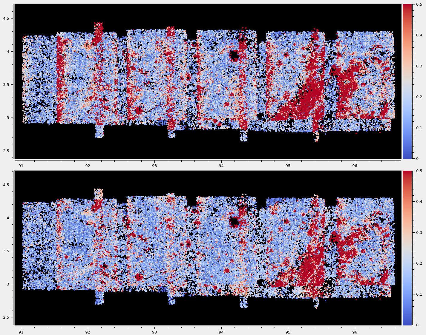
Fig. 12.3 The reprojection errors (pointmap.csv) before (top) and after (bottom)
refinement of distortion. Some outliers are still visible but are harmless.
Dense and uniformly distributed interest points (Section 12.2.4.2) are
strongly suggested, but not used here.
It can be seen that many red vertical patterns are now much attenuated (these
correspond to individual image edges). On the right some systematic errors
are seen (due to the search range in stereo chosen here being too small and
some ridges having been missed). Those do not affect the optimization. Using
mapprojected images would have helped with this. The ultimate check will be
the comparison with LOLA RDR (Fig. 12.4).
Plotted with stereo_gui (Section 16.71.6).
12.2.2.8. Recreation of the stereo DEMs
The new cameras can be used to redo stereo and the DEMs. It is suggested to
use the option --prev-run-prefix in parallel_stereo to
redo only the triangulation operation, which greatly speeds up processing
(see Section 8.31.11 and Section 6.1.7.8).
As before, it is suggested to examine the intersection error and the difference between each produced DEM and the corresponding combined averaged DEM. These errors drop by a factor of about 2 and 1.5 respectively.
12.2.2.9. Comparing to an external ground truth
We solved for intrinsics by constraining against the averaged mosaicked DEM of the stereo pairs produced with initial intrinsics. This works reasonably well if the error due to distortion is somewhat small and the stereo pairs overlap enough that this error gets averaged out in the mosaic.
Ideally, a known accurate external DEM should be used. For example, one could create DEMs using LRO NAC data. Note that many such DEMs would be need to be combined, because LRO NAC has a much smaller footprint.
Should such a DEM exist, before using it instead of the averaged mosaic, the mosaic (or individual stereo DEMs) should be first aligned to the external DEM. Then, the same alignment transform should be applied to the cameras (Section 16.53.14). Then the intrinsics optimization can happen as before.
We use the sparse LOLA RDR dataset (Section 19.11) for final validation. This works well enough because the ground footprint of Kaguya TC is rather large.
Each stereo DEM, before and after intrinsics refinement, is individually aligned to LOLA, and the signed difference to LOLA is found.
 pc_align --max-displacement 50                  \
   --save-inv-transformed-reference-points       \
   dem.tif lola.csv                              \
   -o run_align/run

 point2dem --tr 10   \
  --errorimage       \
  --stereographic    \
  --proj-lon 93.7608 \
  --proj-lat 3.6282  \
  run_align/run-trans_reference.tif

geodiff --csv-format 2:lon,3:lat,4:radius_km     \
  run_align/run-trans_reference-DEM.tif lola.csv \
  -o run_align/run
The pc_align tool is quite sensitive to the value of --max-displacement
(Section 16.53.2). Here it was chosen to be somewhat larger
than the vertical difference between the two datasets to align. That because
KaguyaTC is already reasonably well-aligned.
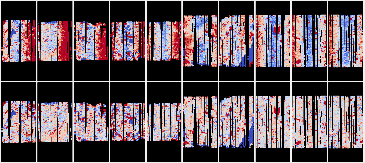
Fig. 12.4 The signed difference between aligned stereo DEMs and LOLA RDR before (top)
and after (bottom) refinement of distortion. (Blue = -20 meters, red = 20
meters.) It can be seen that the warping of the DEMs due to distortion is much
reduced. Plotted with stereo_gui (Section 16.71.6).
12.2.2.10. Handling images with very different illumination
If each stereo pair has consistent illumination, but the illumination is very different between pairs, then the above approach may not work well as tie points could be hard to find. It is suggested to do the initial bundle adjustment per each stereo pair, followed by alignment of the individual produced DEMs to a reference dataset.
Apply the alignment transform to the pairwise bundle-adjusted cameras as well (Section 16.53.14), and use these cameras for the refinement of intrinsics, with the ground constraint being the mosaic of these aligned DEMs.
It is suggested to examine how each aligned DEM differs from the reference, and the same for their mosaic. The hope is that the mosaicking will average out the errors in the individual DEMs.
If a lot of such stereo pairs are present, for the purpose of refinement of intrinsics it is suggested to pick just a handful of them, corresponding to the area where the mosaicked DEM differs least from the reference, so where the distortion artifacts are most likely to have been averaged well.
12.2.3. Mixing frame and linescan cameras
So far we discussed refining the intrinsics for pinhole (frame) cameras, such as in Section 12.2.1.3, and for linescan cameras, such as in Section 12.2.2.
Here we will consider the situation when we have both. It is assumed that the images acquired with these sensors are close in time and have similar illumination. There should be a solid amount of image overlap, especially in the corners of the images whose distortion should be optimized.
It will be illustrated how the presumably more accurate linescan sensor images can be used to refine the intrinsics of the frame sensor.
12.2.3.1. Preparing the inputs
The frame cameras can be in the black-box RPC format (Section 8.22), or any
other format supported by ASP. The cameras can be converted to the CSM format
using cam_gen (Section 16.8.1.4). This will find the best-fit
intrinsics, including the lens distortion.
It is important to know at least the focal length of the frame cameras somewhat accurately. This can be inferred based on satellite elevation and ground footprint.
Once the first frame camera is converted to CSM, the rest of them that are
supposed to be for the same sensor model can borrow the just-solved intrinsic
parameters using the option --sample-file prev_file.json (the cam_gen
manual has the full invocation).
The linescan cameras can be converted to CSM format using cam_gen as well
(Section 16.8.1.5). This does not find a best-fit model, but rather
reads the linescan sensor poses and intrinsics from the input file.
We will assume in this basic example that we have two frame camera images
sharing intrinsics, named frame1.tif and frame2.tif, and two linescan
camera images, for which will not enforce that the intrinsics are shared. They
can even be from different vendors. The linescan intrinsics will be kept fixed.
Assume these files are named linescan1.tif and linescan2.tif. The camera
names will have the same convention, but ending in .json.
12.2.3.2. Initial bundle adjustment
The same approach as in Section 12.2.2.3 can be used. A DEM may be helpful to help figure out which image pairs overlap, but is not strictly necessary.
Ensure consistent order of the images and cameras, both here and in the next
steps. This will guarantee that all generated match files will be used. The
order here will be frame1, frame2, linescan1, linescan2.
It is very strongly suggested to examine the stereo convergence angles (Section 16.5.11.4). At least some of them should be at least 10-15 degrees, to ensure a robust solution.
Also examine the pairwise matches in stereo_gui
(Section 16.71.9.2), the final residuals per camera
(Section 16.5.11.1), and per triangulated point
(Section 16.5.11.5). The latter can be visualized in stereo_gui
(Section 16.71.6). The goal is to ensure well-distributed features,
and that the errors are pushed down uniformly.
Dense interest points produced from stereo are strongly suggested (Section 12.2.4.2). An example using these is in Section 8.8.
12.2.3.3. Evaluation of terrain models
As in Section 12.2.2, it is suggested to create several stereo DEMs after
the initial bundle adjustment. For example, make one DEM for the frame camera
pair, and a second for the linescan one. Use mapprojected images, the
asp_mgm algorithm (Section 6), and a local stereographic
projection for the produced DEMs.
One should examine the triangulation error for each DEM
(Section 14.6.1), and the difference between them with
geodiff (Section 16.26). Strong systematic errors for the frame camera
data will then motivate the next steps.
12.2.3.4. Refinement of the frame camera intrinsics
We will follow closely the recipe in Section 12.2.2. It is suggested to use
for the refinement step the linescan DEM as a constraint (option
--heights-from-dem). If a different DEM is employed, the produced bundle-adjusted
cameras and DEMs should be aligned to it first (Section 16.53.14).
As for Section 12.2.2, we need to create several text files, with each having the names of the images whose intrinsics are shared, and the same for the cameras.
If not sure that the linescan cameras have the same intrinsics, they can be kept in different files. We will keep those intrinsics fixed in either ase.
Assume the previous bundle adjustment was done with the output prefix
ba/run. The files for the next step are created as follows. For the
cameras:
ls ba/run-frame1.adjusted_state.json \
   ba/run-frame2.adjusted_state.json > frame_cameras.txt
ls ba/run-linescan1.adjusted_state.json > linescan1_cameras.txt
ls ba/run-linescan2.adjusted_state.json > linescan2_cameras.txt
and similarly the images. Hence, we have 3 groups of sensors. These
files will be passed to bundle_adjust as follows:
--image-list frame_images.txt,linescan1_images.txt,linescan2_images.txt      \
--camera-list frame_cameras.txt,linescan1_cameras.txt,linescan2_cameras.txt
Use a comma as separator, and no spaces.
We will float the intrinsics for the frame cameras, and keep the linescan intrinsics (but not poses) fixed. This is accomplished with the option:
--intrinsics-to-float '1:focal_length,optical_center,other_intrinsics
                       2:none 3:none'
Optimizing the optical center may not be necessary, as this intrinsic parameter may correlate with the position of the cameras, and these are not easy to separate. Optimizing this may produce an implausible optical center.
Dense matches from disparity are strongly recommended (Section 12.2.4.2).
Some lens distortion parameters can be kept fixed (option
--fixed-distortion-indices).
12.2.3.5. Post-refinement evaluation
New DEMs and intersection error maps can be created. The previous stereo runs
can be reused with the option --prev-run-prefix in parallel_stereo (Section 6.1.7.8).
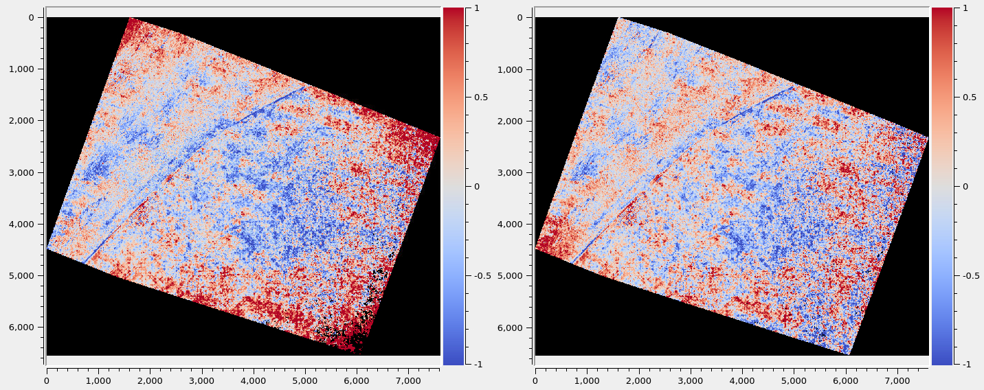
Fig. 12.5 The signed difference between the frame and linescan DEMs before intrinsics refinement (left) and after (right).
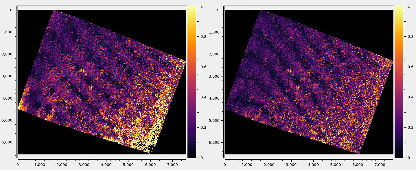
Fig. 12.6 The triangulation error for the frame cameras before refinement of intrinsics (left) and after (right). It can be seen in both figures that systematic differences are greatly reduced.
12.2.4. Custom approaches to interest points
12.2.4.1. Sparse and roughly uniformly distributed interest points
To attempt to create roughly uniformly distributed sparse interest points
during bundle adjustment, use options along the lines --ip-per-tile 1000
--matches-per-tile 500 --max-pairwise-matches 10000.
If the images have very different perspectives, it is suggested to create the interest points based on mapprojected images (Section 12.2.4.3).
Note that if the images are big, this will result in a very large number of potential matches, because a tile has the size of 1024 pixels. (See Section 16.5.13 for the reference documentation for these options.)
To produce sparse interest point matches that are accurate to subpixel level,
use --ip-detect-method 1.
12.2.4.2. Dense and uniformly distributed interest points
Dense and uniformly distributed interest points can be created during stereo (Section 3). If having many images, that will mean many combinations of stereo pairs. A representative set of stereo pairs between all images is usually sufficient.
The resulting interest points will be between the original, unprojected and unaligned images. This is true even when stereo itself is done with mapprojected images.
For each stereo invocation, add options along the lines of:
--num-matches-from-disparity 10000
or:
--num-matches-from-disp-triplets 10000
in order to create such a match file.
The latter option will ensure that, when there are more than two images, a dense subset of features within area of overlap will have corresponding matches in more than two images, with a single triangulated point on the ground for each such matching feature set. If having many such stereo pairs, some triangulated points will be represented with matches in all images.
This can be quite important for bundle adjustment. This number of features for
each triangulated point is the last field in the pointmap.csv report files
(Section 16.5.11.5).
In the latest ASP (Section 2.1), these options are equivalent.
The produced match file name is named along the lines of:
run/run-disp-left__right.match
where left.tif and right.tif are the input images. If these images are
mapprojected, the latest ASP (post version 3.4.0) will instead adjust the match
file name to reflect the original, unprojected image names, as the matches are
between those images.
In either case, the produced match files must be copied from individual stereo
runs to the same directory, and use the standard naming convention for the
original image names (Section 16.5.10.1). The match files must be passed
to bundle_adjust via the --match-files-prefix option. In this example,
the prefix would be run/run-disp.
Invoke bundle_adjust a value of --max-pairwise-matches that is at least
twice the number of matches created here to ensure they are all kept.
A detailed example of using dense matches for bundle adjustment is in Section 8.8.
These options are formally described in Section 17.5.
12.2.4.3. Creating interest point matches using mapprojected images
To make it easier to create interest point matches in situations when the images are very different or taken from very diverse perspectives, the images can be first mapprojected onto a DEM, as then they look a lot more similar. The interest points are created among the mapprojected images, and the matches are transferred to the original images.
This can produce many more interest points when the difference of perspective or scale between images is large. This is done with automatic or manual (GUI) means, as described below.
Given three images A.tif, B.tif, and C.tif,
cameras A.tsai, B.tsai, and C.tsai, and a DEM named dem.tif,
mapproject the images onto this DEM (Section 16.41), obtaining the images
A.map.tif, B.map.tif, and C.map.tif.
for f in A B C; do
    mapproject --tr 1.0 dem.tif $f.tif $f.tsai $f.map.tif
done
The same resolution (option --tr) should be used for all images, which should
be a compromise between the ground sample distance values for these images.
See Section 6.1.7 how how to find a DEM for mapprojection and other details.
12.2.4.3.1. Automatic matching
Bundle adjustment will find interest point matches among the mapprojected images, and transfer them to the original images. Run:
bundle_adjust A.tif B.tif C.tif A.tsai B.tsai C.tsai          \
  --mapprojected-data 'A.map.tif B.map.tif C.map.tif dem.tif' \
  --min-matches 0 -o run/run
This will not recreate any existing match files either for mapprojected images or for unprojected ones. If that is desired, existing match files need to be deleted first.
Add options such as --ip-per-tile 250 --matches-per-tile 250 if needed to
increase the number of interest point matches.
If these images become too many to set on the command line, use the
options --image-list, --camera-list, --mapprojected-data-list
(Section 16.5.13).
The DEM at the end of this option is optional in the latest builds, if it can be looked up from the geoheader of the mapprojected images.
Each mapprojected image stores in its metadata the name of the original image, the camera model, the bundle-adjust prefix, if any, and the DEM it was mapprojected onto. Hence, the above command will succeed even if invoked with different cameras than the ones used for mapprojection, as long as the original cameras are still present and did not change.
If the mapprojected images are still too different for interest point matching among them to succeed, one can try to bring in more images that are intermediate in appearance or illumination between the existing ones, so bridging the gap.
It is suggested to use --mapprojected-data with --auto-overlap-params.
Then, the interest point matching will be restricted to the region of overlap
(expanded by the percentage in the latter option).
Adding --matches-as-txt (Section 19.10) makes both the match file among
the mapprojected images and the unprojected camera-level match file be read and
written in plain text. Externally computed matches among the mapprojected images
can be provided this way, as long as --mapprojected-data is set, so they get
unprojected to the cameras. Such a match file should follow the naming
convention (Section 16.5.10.1). See Section 19.10.5 for more
details.
12.2.4.3.2. Manual matching in the GUI
Alternatively, interest point matching can be done manually in the GUI as follows:
stereo_gui --view-matches A.map.tif B.map.tif C.map.tif run/run
Interest points can be picked by right-clicking on the same feature in each
image, from left to right, and selecting Add match point. Repeat this
process for a different feature. The matches can be saved to disk from the menu.
The bundle adjustment command from above can be invoked to unproject the
matches. Do not forget to first delete first the match files among unprojected
images so that bundle_adjust can recreate them based on the projected
images.
Run:
stereo_gui --view-matches A.tif B.tif C.tif run/run
to check if the interest point matches, that were created using mapprojected
images, were correctly transferred to the original images. Consider using instead
the option --pairwise-matches if some features are not seen in all images.
See Fig. 12.7 for an illustration of this process.
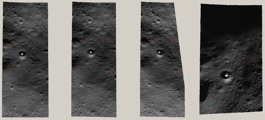
Fig. 12.7 An illustration of how interest points are picked manually for the purpose of bundle adjustment. This is normally not necessary if there exist images with intermediate illumination.
12.2.4.4. Limit extent of interest point matches
To limit the triangulated points produced from interest points to a certain area
during bundle adjustment, two approaches are supported. One is the option
--proj-win, coupled with --proj-str.
The other is using the --weight-image option (also supported by the jitter
solver, Section 16.38). In locations where a given georeferenced weight
image has non-positive or nodata values, triangulated points will be ignored.
Otherwise each pixel reprojection error will be multiplied by the weight closest
geographically to the triangulated point. The effect is to work harder on the
areas where the weight is higher.
Such a weight image can be created from a regular georeferenced image with
positive pixel values as follows. Open it in stereo_gui, and draw on top of
it one or more polygons, each being traversed in a counterclockwise direction,
and with any holes oriented clockwise (Section 16.71.7). Save this shape as
poly.shp, and then run:
cp georeferenced_image.tif aux_image.tif
gdal_rasterize -i -burn -32768 poly.shp aux_image.tif
This will keep the data inside the polygons and set the data outside to this value.
The value to burn should be negative and smaller than any valid pixel value in
the image. To keep the data outside the polygons, omit the -i option.
Then, create a mask of valid values using image_calc (Section 16.33),
as follows:
image_calc -c "max(sign(var_0), 0)" \
 --output-nodata-value var_0        \
 aux_image.tif -o weight.tif
Examine the obtained image in stereo_gui and click on various pixels to
inspect the values.
If the image does not have positive values to start with, those values
can be first shifted up with image_calc.
Various such weight images can be merged with dem_mosaic
(Section 16.20) or the values manipulated with image_calc.
12.2.5. RPC lens distortion
ASP provides a lens distortion model for Pinhole cameras (Section 20.1) that uses Rational Polynomial Coefficients (RPC) of arbitrary degree (Section 20.1.2.8). This can help fit lens distortion where other simpler models cannot.
The tool convert_pinhole_model (Section 16.15) can create
camera models with RPC distortion.
It is very important for the input distortion coefficients to be manually
modified so they are on the order of 1e-7 or more, as otherwise they will be
hard to optimize and may stay small. In the latest builds this is done
automatically by bundle_adjust (option --min-distortion).
See Section 12.2.1.2 and Section 12.2.2 for examples of how to to optimize the lens distortion. An example specifically using RPC is illustrated in Fig. 8.42. It is suggested to use dense interest point matches from disparity (Section 12.2.4.2).
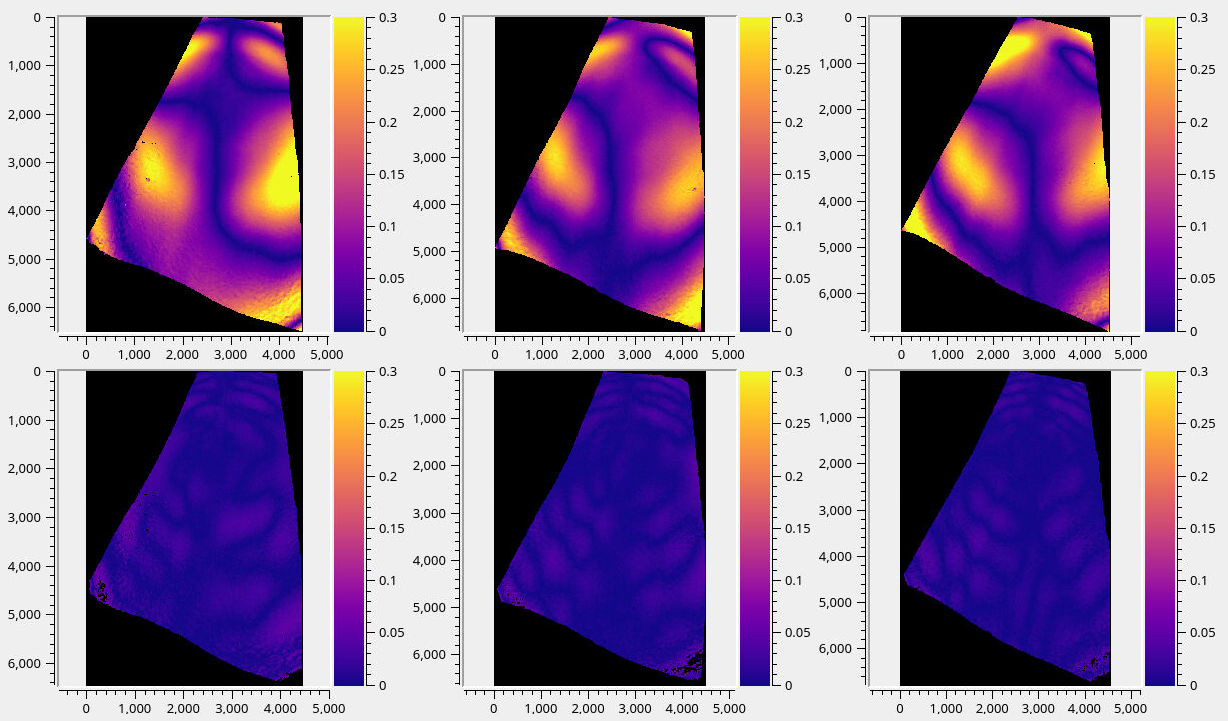
Fig. 12.8 Triangulation error (Section 14.6.1) examples without modeling distortion (top), and after optimizing the lens distortion with RPC of degree 6 (bottom). The dataset for this example was acquired by a drone and had “biradial” distortion.
12.3. Bundle adjustment using ISIS
In what follows we describe how to do bundle adjustment using ISIS’s toolchain. It also serves to describe bundle adjustment in more detail, which is applicable to other bundle adjustment tools as well, including Stereo Pipeline’s own tool.
ASP’s bundle_adjust program can read and write the ISIS control network
format, hence the ASP and ISIS tools can be compared or used together
(Section 16.5.10).
In bundle adjustment, the position and orientation of each camera station are determined jointly with the 3D position of a set of image tie-points points chosen in the overlapping regions between images. Tie points, as suggested by the name, tie multiple camera images together. Their physical manifestation would be a rock or small crater than can be observed across more than one image.
Tie-points are automatically extracted using ISIS’s autoseed and
pointreg (alternatively one could use a number of outside methods
such as the famous SURF [BETG08]). Creating a
collection of tie points, called a control network, is a three step
process. First, a general geographic layout of the points must be
decided upon. This is traditionally just a grid layout that has some
spacing that allows for about 20-30 measurements to be made per image.
This shows up in slightly different projected locations in each image
due to their slight misalignments. The second step is to have an
automatic registration algorithm try to find the same feature in all
images using the prior grid as a starting location. The third step is to
manually verify all measurements visually, checking to insure that each
measurement is looking at the same feature.
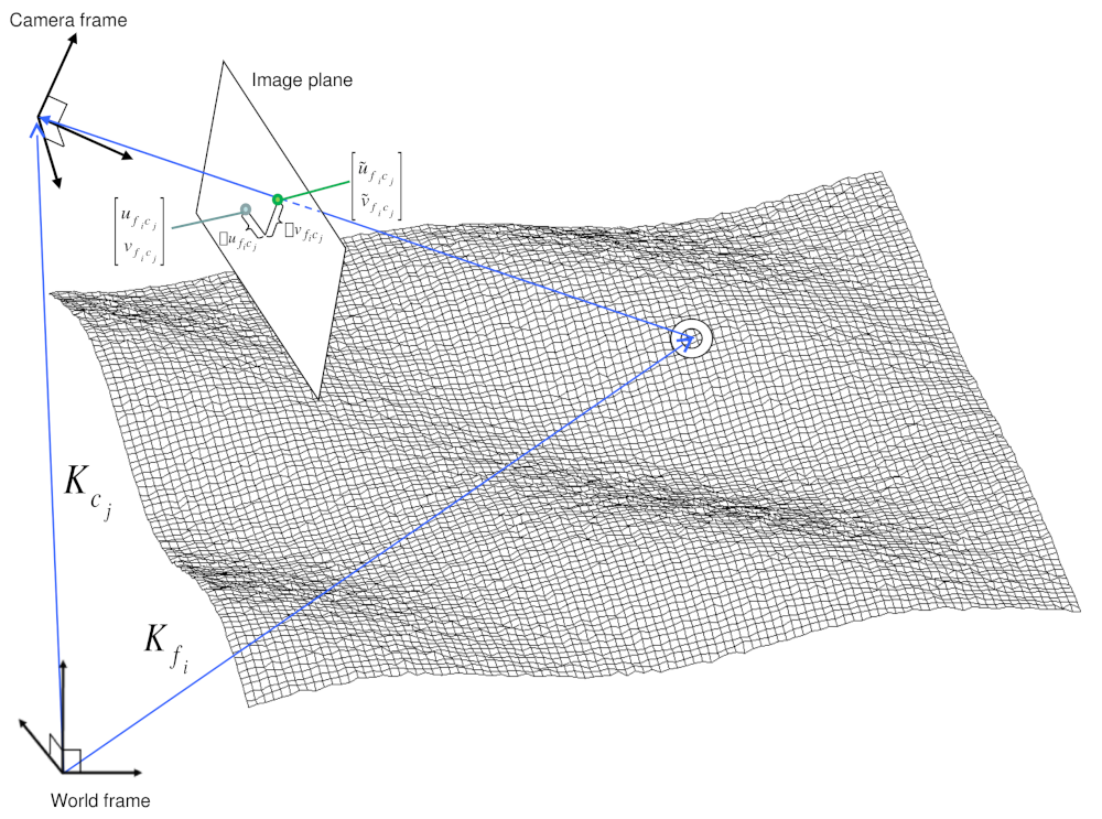
Fig. 12.9 A feature observation in bundle adjustment, from [MWLS09]
Bundle adjustment in ISIS is performed with the jigsaw executable.
It generally follows the method described
in [TMHF00] and determines the best camera
parameters that minimize the projection error given by
where \(I_k\) are the tie points on the image plane, \(C_j\) are the camera parameters, and \(X_k\) are the 3D positions associated with features \(I_k\). \(I(C_j, X_k)\) is an image formation model (i.e. forward projection) for a given camera and 3D point. To recap, it projects the 3D point, \(X_k\), into the camera with parameters \(C_j\).
This produces a predicted image location for the 3D point that is compared against the observed location, \(I_k\). It then reduces this error with the Levenberg-Marquardt algorithm (LMA). Speed is improved by using sparse methods as described in [HZ04], [Kon10], and [CDHR08].
Even though the arithmetic for bundle adjustment sounds clever, there are faults with the base implementation. Imagine a case where all cameras and 3D points were collapsed into a single point. If you evaluate the above cost function, you’ll find that the error is indeed zero. This is not the correct solution if the images were taken from orbit. Another example is if a translation was applied equally to all 3D points and camera locations. This again would not affect the cost function. This fault comes from bundle adjustment’s inability to control the scale and translation of the solution. It will correct the geometric shape of the problem, yet it cannot guarantee that the solution will have correct scale and translation.
ISIS attempts to fix this problem by adding two additional cost functions to bundle adjustment. First of which is
This constrains camera parameters to stay relatively close to their initial values. Second, a small handful of 3D ground control points (Section 16.5.9) can be chosen by hand and added to the error metric as
to constrain these points to known locations in the planetary coordinate frame. A physical example of a ground control point could be the location of a lander that has a well known location. GCPs could also be hand-picked points against a highly regarded and prior existing map such as the THEMIS Global Mosaic or the LRO-WAC Global Mosaic.
Like other iterative optimization methods, there are several conditions that will cause bundle adjustment to terminate. When updates to parameters become insignificantly small or when the error, \({\bf \epsilon}\), becomes insignificantly small, then the algorithm has converged and the result is most likely as good as it will get. However, the algorithm will also terminate when the number of iterations becomes too large in which case bundle adjustment may or may not have finished refining the parameters of the cameras.
12.3.1. Tutorial: Processing Mars Orbital Camera images
This tutorial for ISIS’s bundle adjustment tools is taken from [Mor12a] and [Mor12b]. These tools are not a product of NASA nor the authors of Stereo Pipeline. They were created by USGS and their documentation is available at [Cen].
What follows is an example of bundle adjustment using two MOC images of Hrad
Vallis. We use images E02/01461 and M01/00115, the same as used in
Section 4.2. These images are available from NASA’s PDS (the ISIS
mocproc program will operate on either the IMQ or IMG format files, we use
the .imq below in the example).
Ensure that ISIS and its supporting data is installed, per Section 2.3.1,
and that ISISROOT and ISIS3DATA are set. The string ISIS> is not
part of the shell commands below, it is just suggestive of the fact that we operate
in an ISIS environment.
Fetch the MOC images anc convert them to ISIS cubes.
ISIS> mocproc from=E0201461.imq to=E0201461.cub mapping=no
ISIS> mocproc from=M0100115.imq to=M0100115.cub mapping=no
Note that the resulting images are not map-projected. That because bundle
adjustment requires the ability to project arbitrary 3D points into the camera
frame. The process of map-projecting an image dissociates the camera model from
the image. Map-projecting can be perceived as the generation of a new infinitely
large camera sensor that may be parallel to the surface, a conic shape, or
something more complex. That makes it extremely hard to project a random point
into the camera’s original model. The math would follow the transformation from
projection into the camera frame, then projected back down to surface that ISIS
uses, then finally up into the infinitely large sensor. Jigsaw does not
support this and thus does not operate on map-projected images.
ASP’s bundle_adjust program, however, can create and match features
on mapprojected images, and then project those into the original images
(Section 12.2.4.3).
Before we can dive into creating our tie-point measurements we must finish prepping these images. The following commands will add a vector layer to the cube file that describes its outline on the globe. It will also create a data file that describes the overlapping sections between files.
ISIS> footprintinit from=E0201461.cub
ISIS> footprintinit from=M0100115.cub
ISIS> ls *.cub > cube.lis
ISIS> findimageoverlaps from=cube.lis overlaplist=overlap.lis
At this point, we are ready to start generating our measurements. This
is a three step process that requires defining a geographic pattern for
the layout of the points on the groups, an automatic registration pass,
and finally a manual clean up of all measurements. Creating the ground
pattern of measurements is performed with autoseed. It requires a
settings file that defines the spacing in meters between measurements.
For this example, write the following text into a autoseed.def file.
Group = PolygonSeederAlgorithm
      Name = Grid
      MinimumThickness = 0.01
      MinimumArea = 1
      XSpacing = 1000
      YSpacing = 2000
End_Group
The minimum thickness defines the minimum ratio between the sides of the
region that can have points applied to it. A choice of 1 would define a
square and anything less defines thinner and thinner rectangles. The
minimum area argument defines the minimum square meters that must be in
an overlap region. The last two are the spacing in meters between
control points. Those values were specifically chosen for this pair so
that about 30 measurements would be produced from autoseed. Having
more control points just makes for more work later on in this process.
Run autoseed as follows.
ISIS> autoseed fromlist=cube.lis overlaplist=overlap.lis      \
          onet=control.net deffile=autoseed.def networkid=moc \
          pointid=vallis???? description=hrad_vallis
Note the option pointid=vallis????. It must be used verbatim. This command
will create ids that will look like vallis0001, valis0002, potentially
up to vallis9999. The number of question marks will control hom many
measurements are created. See autoseed’s
manual page for more details.
Inspect this control network with
qnet. Type “qnet” in a terminal, with
no options. A couple of windows will pop up. From the File menu of the
qnet window, click on Open control network and cube list. Open the
file cube.lis. From the same dialog, open control.net.
Click on vallis0001 in the Control Network Navigator window, then click on
view cubes. This will show the illustration below.
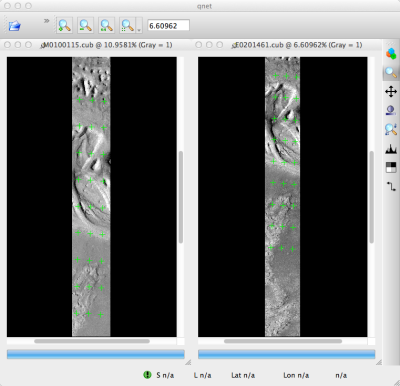
Fig. 12.10 A visualization of the features laid out by autoseed in qnet.
Note that the marks do not cover the same features between images.
This is due to the poor initial SPICE (camera pose) data for MOC images.
The next step is to perform auto registration of these features between the two images using pointreg. This program also requires a settings file that describes how to do the automatic search. Copy the text box below into a autoRegTemplate.def file.
 Object = AutoRegistration
  Group = Algorithm
    Name         = MaximumCorrelation
    Tolerance    = 0.7
  EndGroup

  Group = PatternChip
    Samples = 21
    Lines   = 21
    MinimumZScore = 1.5
    ValidPercent = 80
  EndGroup

  Group = SearchChip
    Samples = 75
    Lines   = 1000
  EndGroup
EndObject
The search chip defines the search range for which pointreg will
look for matching images. The pattern chip is simply the kernel size of
the matching template. The search range is specific for this image pair.
The control network result after autoseed had a large vertical
offset on the order of 500 pixels. The large misalignment dictated the
need for the large search in the lines direction. Use qnet to get an
idea for what the pixel shifts look like in your stereo pair to help you
decide on a search range. In this example, only one measurement failed
to match automatically. Here are the arguments to use in this example of
pointreg.
ISIS> pointreg fromlist=cube.lis cnet=control.net             \
           onet=control_pointreg.net deffile=autoRegTemplate.def
The third step is to verify the measurements in qnet, and, if necessary,
apply manual corrections. Type qnet in the terminal and then open
cube.lis, followed by control_pointreg.net. From the Control Network
Navigator window, click, as before, on the first point, vallis0001. That opens
a third window called the Qnet Tool. That window will allow you to play a flip
animation that shows alignment of the feature between the two images. Correcting
a measurement is performed by left clicking in the right image, then clicking
Save Measure, and finally finishing by clicking Save Point.
In this tutorial, measurement 0025 ended up being incorrect. Your number may vary if you used different settings than the above or if MOC SPICE (camera pose) data has improved since this writing. When finished, go back to the main Qnet window. Save the final control network as control_qnet.net by clicking on File, and then Save As.
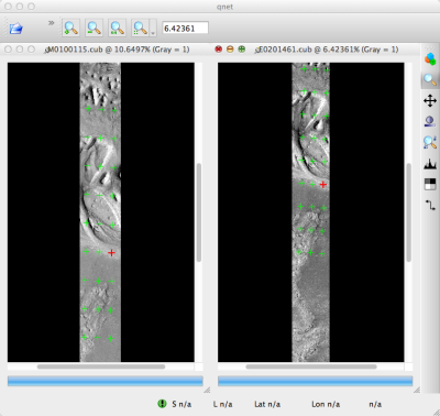
Fig. 12.11 A visualization of the features after manual editing in qnet.
Note that the marks now appear in the same location between images.
Once the control network is finished, it is finally time to start bundle
adjustment. Here’s how jigsaw is called:
ISIS> jigsaw                                  \
        fromlist           = cube.lis         \
        update             = yes              \
        twist              = no               \
        radius             = yes              \
        point_radius_sigma = 1000             \
        cnet               = control_qnet.net \
        onet               = control_ba.net
The update option defines that we would like to update the camera pointing, if
our bundle adjustment converges. The twist = no option says to not solve for
the camera rotation about the camera bore. That property is usually very well
known as it is critical for integrating an image with a line-scan camera. The
radius = yes setting means that the radius of the 3D features can be solved
for. Using radius = no will force the points to use height values from
another source, usually LOLA or MOLA. The point_radius_sigma option defines
the uncertainty of the radius of the 3D points, in units of meter.
The above command will print out diagnostic information from every iteration of the optimization algorithm. The most important feature to look at is the sigma0 value. It represents the mean of pixel errors in the control network. In our run, the initial error was 1065 pixels and the final solution had an error of 1.1 pixels.
Producing a DEM using the newly created camera corrections is the same
as covered in the Tutorial. When using jigsaw, it modifies
a copy of the SPICE data that is stored internally to the cube file.
Thus, when we want to create a DEM using the correct camera geometry, no extra
information needs to be given to parallel_stereo since it is already
contained in the camera files.
More information is in the jigsaw documentation.
See Section 16.5.10 for how to use the resulting control network in
bundle_adjust.
In the event a mistake has been made, spiceinit will overwrite the SPICE
data inside a cube file and provide the original uncorrected camera pointing.
It can be invoked on each cub file as:
ISIS> spiceinit from=image.cub
In either case, then one can run stereo:
ISIS> parallel_stereo              \
        --stereo-algorithm asp_mgm \
        --subpixel-mode 9          \
        E0201461.cub M0100115.cub  \
        stereo/run
See Section 6 for how how to improve the quality of stereo correlation results (at the expense of speed), how to create a DEM, etc.
12.4. Using the ISIS cnet format in ASP
ASP’s bundle_adjust program can read and write control networks in the ISIS
format (and they are read by jitter_solve as well). A basic overview of how
this works is in Section 16.5.10.2. This section provides more details.
A priori surface points will be read and written back (they may change only in special cases, see below). Adjusted surface points will be read, optimized, then written back.
For constrained surface points, the constraint will be relative to the a priori surface points. These will be used with sigmas from adjusted surface points, as the a priori sigmas are on occasion negative, and likely the adjusted sigmas are more up-to-date.
Constrained surface points are treated as GCP in bundle_adjust
(Section 16.5.9), so smaller sigmas result in more weight given to the
discrepancy betwen surface points being optimized and a priori surface points.
Fixed surface points will be set to the a priori values and kept fixed during the optimization.
Any input points that are flagged as ignored or rejected will be treated as outliers and will not be used in the optimization. They will be saved the same way. Additional points may be tagged as outliers during optimization. These will be flagged as ignored and rejected on output.
Partially constrained points will be treated as free points during the optimization, but the actual flags will be preserved on saving.
Control measure sigmas are read and written back. They will be used in the
optimization. If not set in the input file, they will be assigned the value 1.0
by bundle_adjust, and it is this value that will be saved.
Pixel measurements will have 0.5 subtracted on input, and then added back on output.
If bundle_adjust is invoked with GCP files specified separately in ASP’s GCP
format, the GCP will be appended to the ISIS control network and then saved
together with it. These points will be treated as constrained (with provided
sigmas and a priori surface values), unless the sigmas are set to the precise
value of 1e-10, or when the flag --fix-gcp-xyz is used, in which case they
will be treated as fixed both during optimization and when saving to the ISIS
control network file. (For a small value of sigma, GCP are practically fixed in
either case.)
Using the bundle_adjust options --initial-transform and
--input-adjustments-prefix will force the recomputation of a priori points
(using triangulation), as these options can drastically change the cameras.
A priori points will change if --heights-from-dem is used
(Section 12.2.1.3). The sigmas will be set to what is provided via the
--heights-from-dem-uncertainty option.
If exporting match files from an ISIS control network (option
--output-cnet-type match-files), constrained and fixed points won’t be
saved, as ASP uses GCP files for that. Saved match files will have the rest of
the matches, and clean match files will have only the inliers. Any sigma values
and surface points from the control network will not be saved.