14. Error propagation¶

At the triangulation stage, parallel_stereo can propagate the errors (uncertainties, standard deviations, covariances) from the input cameras, computing the horizontal and vertical standard deviation (stddev) of the uncertainty for each triangulated point. This is enabled with the option --propagate-errors (Section 17.6).

The produced uncertainties are then propagated from the point cloud to the produced DEM (Section 14.3).

14.1. The input uncertainties¶

The input uncertainties can be either numbers that are passed on the command line, or, otherwise, for a few camera models, they can be read from the camera files.

If the option --horizontal-stddev is set, with two positive numbers as values, representing the left and right camera stddev of position uncertainty in the local horizontal ground plane having the triangulated point, then these values will be used. The input stddev values are measured in meters. This functionality works with any cameras supported by ASP.

If this option is not set, the following strategies are used:

For Pleiades 1A/1B linescan camera models (Section 8.21) (but not for NEO, Section 8.21.3) the ACCURACY_STDV field is read from the “DIM” XML file for each camera (in the Absolute Horizontal Accuracy section of the camera model), and it is used as the horizontal stddev.

For Maxar (DigitalGlobe) RPC cameras (Section 8.19), the values ERRBIAS and ERRRAND are read from each camera model file. The square root of sum of squares of these quantities is the input horizontal stddev for a camera.

For Maxar (DigitalGlobe) linescan cameras (Section 5), the inputs are the satellite position and orientation covariances, read from the EPHEMLIST and ATTLIST fields. These are propagated from the satellites to the ground and then through triangulation.

For datasets with a known CE90 measure, or in general a \(CE_X\) measure, where \(X\) is between 0% and 100%, use the --horizontal-stddev option, with values computed using the formula:

\[StdDev = CE_X/\sqrt{-2 \ln(1-X/100.0)}\]

(reference).

In all cases, the error propagation takes into account whether the cameras are bundle-adjusted or not (Section 16.5), and if the images are mapprojected (Section 6.1.7).

14.2. Produced uncertainty for triangulated points¶

The triangulation covariance matrix is computed in the local North-East-Down (NED) coordinates at each nominal triangulated point, and further decomposed into the horizontal and vertical components (Section 14.7).

The square root is taken, creating the stddev, which are saved as the 5th and 6th band in the point cloud (*-PC.tif file, Section 19). Running gdalinfo (Section 16.24) on the point cloud will show some metadata describing each band in that file.

The computed stddev values are in units of meter.

14.3. Propagation of uncertainties to the DEM¶

The stddev values in the point cloud can then be gridded with point2dem (Section 16.55) with the option --propagate-errors, using the same algorithm as for computing the DEM heights.

Example:

point2dem --t_srs <projection string> --tr <grid size> \
  --propagate-errors run/run-PC.tif

This will produce the files run/run-HorizontalStdDev.tif and run/run-VerticalStdDev.tif alongside the output DEM, run/run-DEM.tif.

In all these files the values are in units of meter.

14.4. Implementation details¶

Note that propagating the errors subtly changes the behavior of stereo triangulation, and hence also of the output DEM. Triangulated points are saved with a float precision of 1e-8 meters (rather than the usual 1e-3 meters or so, Section 17.5), to avoid creating step artifacts later when gridding the rather slowly varying propagated errors.

When error propagation is enabled, the triangulated point cloud stores 6 bands instead of the usual 4 (Section 19), and the LZW compression is somewhat less efficient since more digits of precision are stored. The size of the point cloud roughly doubles. This does not affect the size of the DEM, but its values and extent may change slightly.

14.5. What the produced uncertainties are not¶

The horizontal and vertical stddev values created by stereo triangulation and later gridded by point2dem measure the uncertainty of each nominal triangulated point, given the uncertainties in the input cameras.

This is not the discrepancy between this point’s location as compared to to a known ground truth. If the input cameras are translated by the same amount in the ECEF coordinate system, the triangulated point position can change a lot, but the produced uncertainties will change very little. To estimate and correct a point cloud’s geolocation invoke an alignment algorithm (Section 16.52).

The produced uncertainties are not a measure of the pointing accuracy (Section 11.4.1). Whether the rays from the cameras meet at the nominal triangulated point perfectly, or their closest distance is, for example, 5 meters, the produced uncertainties around the nominal point will be about the same. See a comparison between these errors in Fig. 14.1 and Fig. 14.2.

The pointing accuracy can be improved by using bundle adjustment (Section 16.5) and solving for jitter (Section 16.37).

14.6. Example¶

For Maxar (DigitalGlobe) linescan cameras:

 parallel_stereo --alignment-method local_epipolar \
   --stereo-algorithm asp_mgm --subpixel-mode 9    \
   -t dg --propagate-errors                        \
   left.tif right.tif left.xml right.xml
   run/run
point2dem --tr 1.6                                            \
  --t_srs "+proj=utm +zone=13 +datum=WGS84 +units=m +no_defs" \
  --propagate-errors run/run-PC.tif

The projection and grid size above are dependent on the dataset.

Alternatively, the input horizontal stddev values for the cameras can be set as:

--horizontal-stddev 1.05 1.11

Then these will be used instead. This last approach works for any orbital camera model supported by ASP (Section 8).

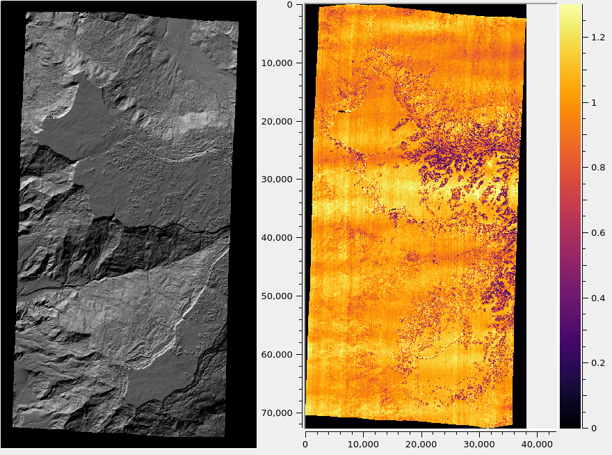
_images/grand_mesa_dem_intersection_err.png — Fig. 14.1 A hillshaded DEM created with DigitalGlobe WorldView images for Grand Mesa, Colorado (left), and the triangulation error (Section 11.4.1) in meters (right). The input images were mapprojected (Section 6.1.7). No bundle adjustment was used. Jitter (Section 16.37) is noticeable.¶

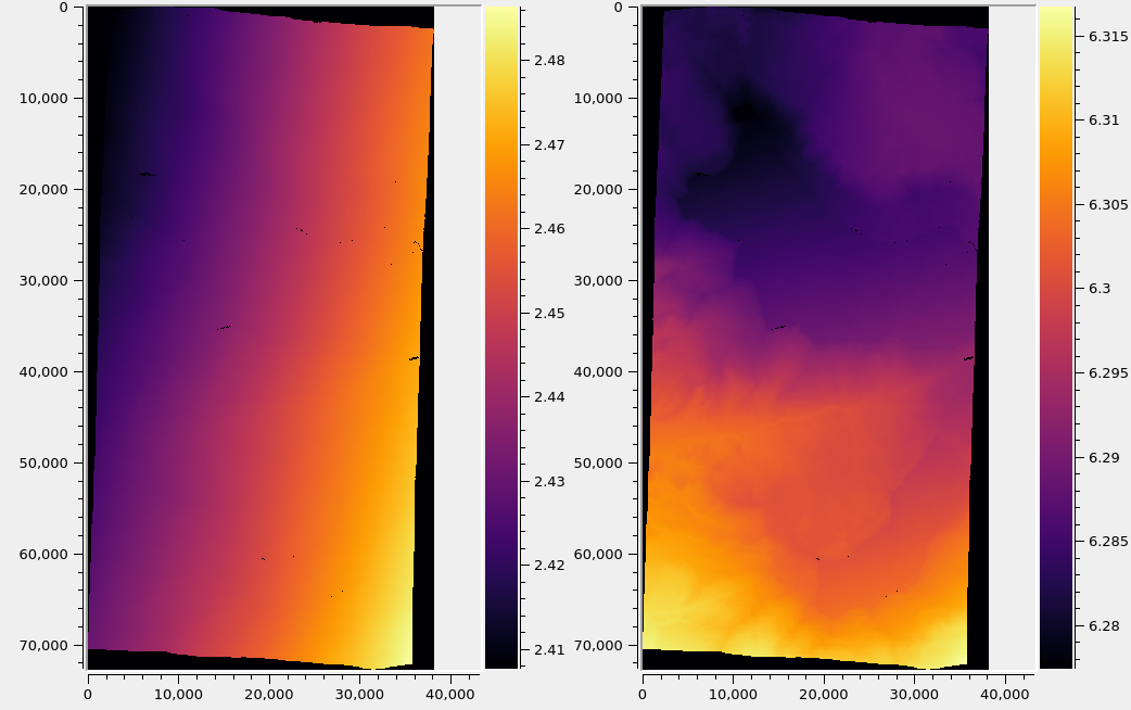
_images/horizontal_vertical_error.png — Fig. 14.2 Produced horizontal and vertical stddev values (left and right) for the same dataset. It can be seen from the scales (units are in meter) and comparing with Fig. 14.1 that these errors vary little overall, and depend more on the geometry of the stereo pair than the underlying terrain. See Section 14.5 for a discussion.¶

14.7. Definitions¶

The vertical variance of a triangulated point is defined as the lower-right corner of the 3x3 NED covariance matrix (since x=North, y=East, z=Down).

To find the horizontal variance component, consider the upper-left \(2 \times 2\) block of that matrix. Geometrically, the horizontal covariances represent an ellipse. The radius of the circle with the same area is found, which is the square root of the product of ellipse semiaxes, which is the product of the eigenvalues of this symmetric matrix, or its determinant. So, the the horizontal component of the covariance is defined as the square root of the upper-left \(2 \times 2\) bock of the NED covariance matrix.

The square root is taken to go from variance to stddev.

14.8. Theory¶

According to the theory of propagation of uncertainty, given a function \(y = f(x)\) between multi-dimensional spaces, the covariances of the inputs and outputs are related via

\[Cov_Y = J Cov_X J^T\]

Here, \(J\) is the Jacobian of the function \(f\) and \(J^T\) is its transpose. It is assumed that the uncertainties are small enough that this function can be linearized around the nominal location.

For this particular application, the input variables are either the coordinates in the local horizontal ground plane having the triangulated point (two real values for each camera), or the satellite positions and orientations (quaternions), which are 7 real values for each camera. The output is the triangulated point in the local North-East-Down coordinates.

If the input uncertainties are stddev values, then these are squared, creating variances, before being propagated (then converted back to stddev values at the last step).

The Jacobian was computed using centered finite differences, with a step size of 0.01 meters for the position and 1e-6 for the (normalized) quaternions. The computation was not particularly sensitive to these step sizes. A much smaller position step size is not recommended, since the positions are on the order of 7e6 meters, (being measured from planet center) and because double precision computations have only 16 digits of precision.

14.9. Validation for Maxar (DigitalGlobe) linescan cameras¶

The horizontal stddev values propagated through triangulation are on the order of 3 meters.

The obtained vertical stddev varies very strongly with the convergence angle, and is usually, 5-10 meters, and perhaps more for stereo pairs with a convergence angle under 30 degrees.

The dependence on the convergence angle is very expected. But these numbers appear too large given the ground sample distance of DigitalGlobe WorldView cameras. We are very confident that they are correct. The results are so large is because of the input orientation covariances (the relative contribution of input position and orientation covariances can be determined with the options --position-covariance-factor and --orientation-covariance-factor).

The curious user can try the following independent approach to validate these numbers. The linescan camera files in XML format have the orientations on lines with the ATTLIST field. The numbers on that line are measurement index, then the quaternions (4 values, in order x, y, z, w) and the upper-right half of the 4x4 covariance matrix (10 numbers, stored row-wise).

The w variance (the last number), can be, for example, on the order of 6.3e-12. Its square root, the standard deviation, which is 2.5e-6 or so, is the expected variability in the w component of the quaternion.

Fetch and save the Python script bias_dg_cam.py. Invoke it as:

python bias_dg_cam.py --position-bias "0 0 0" \
  --orientation-bias "0 0 0 2.5e-6"           \
  -i left.xml -o left_bias.xml
python bias_dg_cam.py --position-bias "0 0 0" \
  --orientation-bias "0 0 0 -2.5e-6"          \
  -i right.xml -o right_bias.xml

This will bias the positions and quaternions in the camera files by the given amounts, creating left_bias.xml and right_bias.xml. Note that values with different sign were used in the two camera files. It is instructive to compare the original and produced camera files side-by-side, and see the effect of using a different sign and magnitude for the biases.

Then, parallel_stereo can be run twice, with different output prefixes, first with the original cameras, and then the biased ones, in both cases without propagation of errors. Use --left-image-crop-win and --right-image-crop-win (Section 16.67) to run on small clips only.

The created DEMs (with nominal and then with biased cameras) can have their heights compared using the geodiff --absolute command (Section 16.25). We found a height difference that is very similar to the vertical standard deviation produced earlier.