3. How ASP works

The Stereo Pipeline package contains command-line and GUI programs that convert a stereo pair consisting of images and cameras into a 3D “point cloud” image. This is an intermediate format that can be passed along to one of several programs that convert a point cloud into a mesh for 3D viewing, a gridded digital terrain model (DTM) for GIS purposes, or a LAS/LAZ point cloud.

There are a number of ways to fine-tune parameters and analyze the results, but ultimately this software suite takes images and builds models in a mostly automatic way.

To create a point cloud file, not necessarily of best quality, for now, one simply passes two image files to the parallel_stereo (Section 16.52) command:

parallel_stereo --stereo-algorithm asp_bm \
  left_image.cub right_image.cub results/run

Higher quality results, at the expense of more computation, can be achieved by running:

parallel_stereo --alignment-method affineepipolar \
  --stereo-algorithm asp_mgm --subpixel-mode 3    \
  left_image.cub right_image.cub results/run

The option --subpixel-mode 9 is faster and still creates decent results (with asp_mgm/asp_sgm). The best quality will likely be obtained with --subpixel-mode 2, but this is even more computationally expensive.

It is very recommended to read Section 6, which describes other alignment methods and stereo algorithms.

Then normally one would create a DEM (Section 16.57):

point2dem --auto-proj-center results/run-PC.tif

Here it is assumed that the PATH and ISISDATA environmental variables have been set, as shown in Section 2.

The .cub file format is used for non-Earth images (Section 4.2). For Earth, the images are usually in the .tif format (Section 5).

The above commands will decompose the images in tiles to run in parallel, potentially on multiple machines (Section 16.52).

Or the stereo_gui frontend can be invoked, with the same options, as described in Section 16.70. This tool makes it possible to manually select smaller clips on which to run parallel_stereo.

The string results/run is an arbitrary output prefix. All parallel_stereo output files will be in the results directory and start with output. See Section 19 for the list of output files.

A a visualizable mesh can be made with the following command (the results/run-PC.tif and results/run-L.tif files are created by the parallel_stereo program above):

point2mesh results/run-PC.tif results/run-L.tif

Visualization is further discussed in Section 6.2.

A produced DEM may need to be aligned to some pre-existing reference (Section 16.54).

If the positions, orientations, or intrinsics of the cameras are not known well, then bundle adjustment may be necessary (Section 12).

What follows are two examples of processing non-Earth data. An example using Earth data is in Section 5. The various stereo algorithms are discussed in Section 6. More examples can be found in Section 8.

4. Tutorial: Processing planetary data (non-Earth)

4.1. Lightning-fast example using Lunar images

This example is designed to have the user create useful results with ASP using Lunar data 10 minutes or less. It does not require a download of ISIS or ISIS data (which can be a couple of hundreds of GB) because it uses the CSM camera model (Section 8.11). The steps to process it are as follows:

• Get ASP per the installation page (Section 2).

• Fetch the LRO NAC example with wget, and extract it as:

  tar xfv LRONAC_example.tar
  

• Start stereo_gui (Section 16.70) with a selection of clips:

  cd LRONAC_example
  stereo_gui M181058717LE_crop.cub M181073012LE_crop.cub \
    M181058717LE.json M181073012LE.json                  \
    --alignment-method local_epipolar                    \
    --left-image-crop-win 2259 1196 900 973              \
    --right-image-crop-win 2432 1423 1173 1218           \
    --stereo-algorithm asp_mgm --subpixel-mode 9         \
    run/run
  

The crop windows from above will show up as red rectangles.

Choose from the menu Run -> Run parallel_stereo. When finished, quit the GUI and run point2dem (Section 16.57) from the command line:

point2dem --auto-proj-center  \
  --errorimage run/run-PC.tif \
  --orthoimage run/run-L.tif

Open the computed DEM and orthoimage as:

stereo_gui run/run-DEM.tif run/run-DRG.tif

Right-click on the DEM on the left and choose to toggle hillshading to show the DEM hillshaded. See the figure below for the output.

How to get higher quality results is described in Section 6.

For other examples, see Section 8.

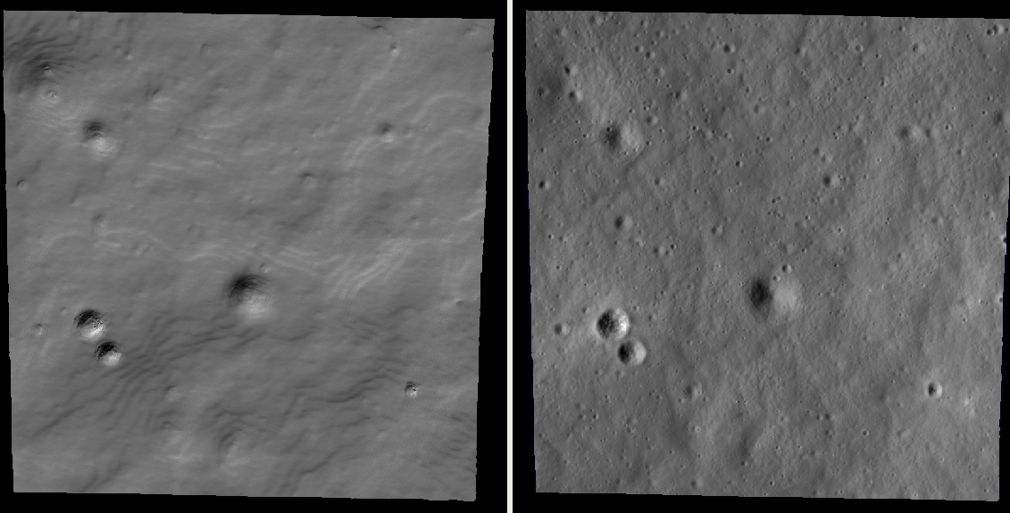
Fig. 4.1 Example of produced DEM and orthoimage using LRO NAC stereo pair M181058717LE and M181073012LE and CSM cameras. How to obtain and prepare the inputs is discussed in Section 8.7. Mapprojection can eliminate the staircasing artifacts (Section 6.1.7).

4.2. Example using Mars MOC images

The data set that is used in the tutorial and examples below is a pair of Mars Orbital Camera (MOC) [MalinDanielsonIngersoll+92, MalinEdgett01] images whose PDS Product IDs are M01/00115 and E02/01461. This data can be downloaded from the PDS directly, or they can be found in the examples/MOC directory of your Stereo Pipeline distribution.

These raw PDS images (M0100115.imq and E0201461.imq) need to be converted to .cub files and radiometrically calibrated. You will need to be in an ISIS environment (Section 2.3.1), usually via a conda activate command which sets the ISISROOT and ISISDATA environment variables; we will denote this state with the ISIS> prompt.

Then you can use the mocproc program, as follows:

ISIS> mocproc from=M0100115.imq to=M0100115.cub Mapping=NO
ISIS> mocproc from=E0201461.imq to=E0201461.cub Mapping=NO

There are also Ingestion and Calibration parameters whose defaults are YES which will bring the image into the ISIS format and perform radiometric calibration. By setting the Mapping parameter to NO, the resultant file will be an ISIS cube file that is calibrated, but not map-projected. Note that while we have not explicitly run spiceinit, the Ingestion portion of mocproc quietly ran spiceinit for you (you’ll find the record of it in the ISIS Session Log, usually written out to a file named print.prt). Fig. 4.2 shows the results at this stage of processing.

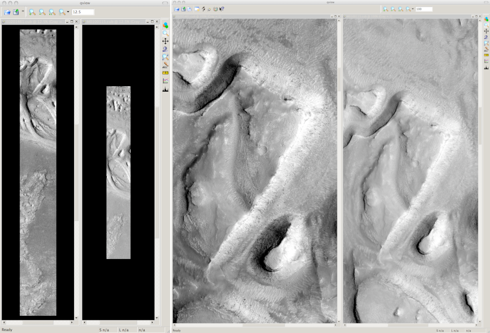
Fig. 4.2 This figure shows E0201461.cub and M0100115.cub open in ISIS’s qview program. The view on the left shows their full extents at the same zoom level, showing how they have different ground scales. The view on the right shows both images zoomed in on the same feature.

See Section 8 for many solved examples, including how to preprocess the data with tools specific for each mission.

Once the .cub files are obtained, it is possible to run parallel_stereo right away, and create a DEM:

ISIS> parallel_stereo E0201461.cub M0100115.cub   \
        --alignment-method affineepipolar         \
        -s stereo.default.example results/output
ISIS> point2dem --auto-proj-center                \
        results/output-PC.tif

In this case, the first thing parallel_stereo does is to internally align (or rectify) the images, which helps with finding stereo matches. Here we have used affineepipolar alignment. Other alignment methods are described in Section 6.1.2.

If your data has steep slopes, mapprojection can improve the results. See Section 6.1.7 and Section 14.6.2.

When creating a DEM, it is suggested to use a local projection (Section 16.57.1).

See Section 6 for a more in-depth discussion of stereo algorithms.

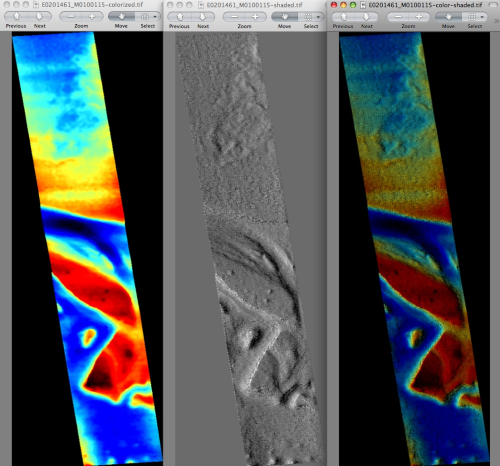
Fig. 4.3 The produced colorized DEM, the shaded relief image, and the colorized hillshade. See Section 6.2.2 for more details.

5. Tutorial: Processing Earth images

In this chapter we will focus on how to process Earth images, or more specifically DigitalGlobe (Maxar) WorldView and QuickBird images. This example is different from the one in the previous chapter in that at no point will we be using ISIS utilities. This is because ISIS only supports NASA instruments, while most Earth images comes from commercial providers.

In addition to DigitalGlobe/Maxar’s satellites, ASP supports any Earth images that uses the RPC camera model format. How to process such data is described in Section 8.18, although following this tutorial may still be insightful even if your data is not from DigitalGlobe/Maxar.

If this is your first time running ASP, it may be easier to start with ASTER data (Section 8.16), as its images are free and much smaller than DigitalGlobe’s. A ready-made example having all inputs, outputs, and commands, is provided there.

DigitalGlobe provides images from QuickBird and the three WorldView satellites. These are the hardest images to process with Ames Stereo Pipeline because they are exceedingly large, much larger than HiRISE images. The GUI (Section 16.70) can be used to run stereo on just a portion of the images.

The camera information for DigitalGlobe/Maxar images is contained in an XML file for each image. In addition to the exact linear camera model, the XML file also has its RPC approximation. In this chapter we will focus only on processing data using the linear camera model. For more detail on RPC camera models we refer as before to Section 8.18.

Our implementation of the Digital Globe linear camera model accounts for the sensor geometry, velocity aberration and atmospheric refraction (Section 5.9).

In the next two sections we will show how to process unmodified and map-projected variants of WorldView images. These images represent a non-ideal problem for us since this is an urban location, but at least you should be able to download these images yourself and follow along.

5.1. Supported products

ASP can only process DigitalGlobe / Maxar Level 1B satellite images, and there is experimental support for View-Ready OR2A images (see Section 6.1.7.9). ASP cannot handle images that are orthorectified onto a DEM. See the list of products.

5.2. Processing raw

After you have downloaded the example stereo images of Stockholm, you will find a directory titled:

056082198020_01_P001_PAN

It has a lot of files and many of them contain redundant information just displayed in different formats. We are interested only in the TIF or NTF images and the similarly named XML files.

Some WorldView folders will contain multiple image files. This is because DigitalGlobe/Maxar breaks down a single observation into multiple files for what we assume are size reasons. These files have a pattern string of “_R[N]C1-“, where N increments for every subframe of the full observation. The tool named dg_mosaic (Section 16.21) can be used to mosaic such a set of sub-observations into a single image file and create an appropriate camera file:

dg_mosaic 12FEB16101327*TIF --output-prefix 12FEB16101327

and analogously for the second set. See Section 16.21 for more details. The parallel_stereo program can use either the original or the mosaicked images. This sample data only contains two image files so we do not need to use dg_mosaic.

Since we are ingesting these images raw, it is strongly recommended that you use affine epipolar alignment to reduce the search range. Commands:

parallel_stereo -t dg --stereo-algorithm asp_mgm      \
  --subpixel-mode 9 --alignment-method affineepipolar \
  12FEB16101327.r50.tif 12FEB16101426.r50.tif         \
  12FEB16101327.r50.xml 12FEB16101426.r50.xml         \
  run/run
point2dem --auto-proj-center run-PC.tif

As discussed in Section 3, one can experiment with various tradeoffs of quality versus run time by using various stereo algorithms, and use stereo in parallel or from a GUI. For more details, see Section 6.

How to create a DEM and visualize the results of stereo is described in Section 6.2. Choosing a projection is discussed in Section 16.57.1.

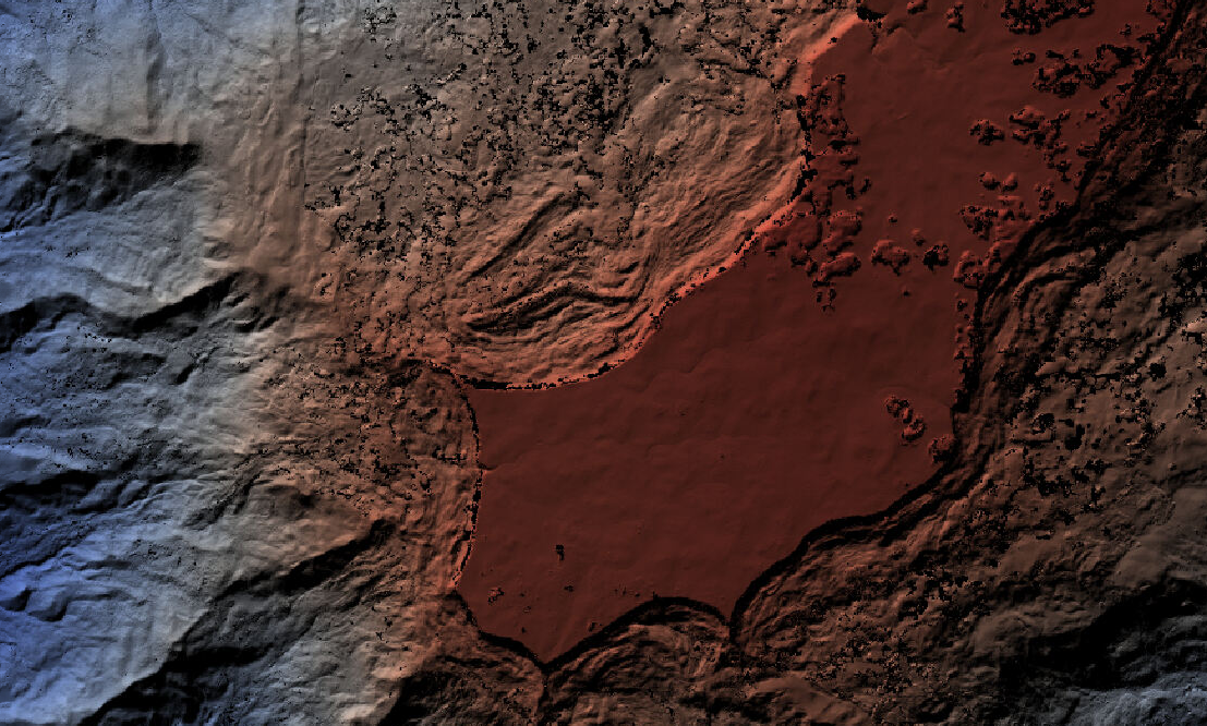
Fig. 5.1 A colorized and hillshaded terrain model for Grand Mesa, Colorado, produced with WorldView images, while employing mapprojection (Section 6.1.7).

It is important to note that we could have performed stereo using the approximate RPC model instead of the exact linear camera model (both models are in the same XML file), by switching the session in the parallel_stereo command above from -t dg to -t rpc. The RPC model is somewhat less accurate, so the results will not be the same, in our experiments we’ve seen differences in the 3D terrains using the two approaches of 5 meters or more.

Many more stereo processing examples can be found in Section 8.

5.3. Processing map-projected images

ASP computes the highest quality 3D terrain if used with images map-projected onto a low-resolution DEM that is used as an initial guess. This process is described in Section 6.1.7.

5.4. Dealing with clouds

Clouds can result in unreasonably large disparity search ranges and a long run-time. It is then suggested to mapproject the images (Section 6.1.7).

With our without mapprojection, one can reduce the computed search range via --max-disp-spread (Section 17). Use this with care. Without mapprojection and with steep terrain, the true spread of the disparity can, in rare cases, reach a few thousand pixels. This is best used with mapprojected images, when it is likely to be under 150-200, or even under 100.

If a reasonable DEM of the area of interest exists, the option --ip-filter-using-dem can be used to filter out interest points whose heights differ by more than a given value than what is provided by that DEM. This should reduce the search range. Without a DEM, the option --elevation-limit can be used and should have a similar effect.

Another option (which can be used in conjunction with the earlier suggestions) is to tighten the outlier filtering in the low-resolution disparity D_sub.tif (Section 19), for example, by setting --outlier-removal-params 70 2 from the default 95 3 (Section 17). Note that decreasing these a lot may also filter out valid steep terrain.

If a run failed because of a large disparity search range, D_sub.tif should be deleted, parameters adjusted as above, and one should run stereo_corr with the same arguments that parallel_stereo was run before (except those used for tiling and number of processes, etc.), while adding the option --compute-low-res-disparity-only. Then examine the re-created D_sub.tif with disparitydebug (Section 16.23) and the various search ranges printed on screen.

The D_sub.tif file can be created from a DEM (Section 14.3.2).

When D_sub.tif is found to be reasonable, parallel_stereo should be re-run with the option --resume-at-corr.

See also Section 6.1.9 which offers further suggestions for how to deal with long run-times.

5.5. Handling CCD boundary artifacts

DigitalGlobe/Maxar WorldView images [Glo] may exhibit slight subpixel artifacts which manifest themselves as discontinuities in the 3D terrain obtained using ASP. We provide a tool named wv_correct, that can largely correct such artifacts for World View-1 and WorldView-2 images for most TDI.

Note that Maxar (DigitalGlobe) WorldView-2 images with a processing date (not acquisition date) of May 26, 2022 or newer have much-reduced CCD artifacts, and for those this tool will in fact make the solution worse, not better. This does not apply to WorldView-1, 3, or GeoEye-1.

This tool can be invoked as follows:

wv_correct image_in.ntf image.xml image_out.tif

The corrected images can be used just as the originals, and the camera models do not change. When working with such images, we recommend that CCD artifact correction happen first, on original un-projected images. Afterward images can be mosaicked with dg_mosaic, map-projected, and the resulting data used to run stereo and create terrain models.

This tool is described in Section 16.76, and an example of using it is in Fig. 5.2.

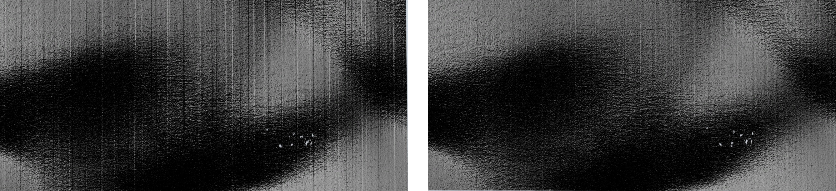
Fig. 5.2 Example of a hill-shaded terrain obtained using stereo without (left) and with (right) CCD boundary artifact corrections applied using wv_correct.

5.6. Images lacking large-scale features

See Section 14.3.2 and Section 14.3.3 for suggestions on how to deal with images that lack large-scale features, such as when the images have a lot of snow.

5.7. Jitter

Another source of artifacts in linescan cameras, such as from DigitalGlobe, is jitter. ASP can solve for it using a jitter solver (Section 16.39).

5.8. Multi-spectral images

In addition to panchromatic (grayscale) images, the DigitalGlobe/Maxar satellites also produce lower-resolution multi-spectral (multi-band) images. Stereo Pipeline is designed to process single-band images only. If invoked on multi-spectral data, it will quietly process the first band and ignore the rest. To use one of the other bands it can be singled out by invoking dg_mosaic (Section 5.2) with the --band <num> option. We have evaluated ASP with DigitalGlobe/Maxar’s multi-spectral images, but support for it is still experimental. We recommend using the panchromatic images whenever possible.

5.9. Implementation details

WorldView linescan cameras use the CSM model (Section 8.11) internally. The session name must still be -t dg, -t dgmaprpc, etc., rather than -t csm, -t csmmapcsm, etc.

Bundle adjustment (Section 16.5) and solving for jitter (Section 16.39) produce optimized camera models in CSM’s model state format (Section 8.11.6). These can be used just as the original cameras, but with the option -t csm. Alternatively, the bundle_adjust .adjust files can be used with the original cameras.

Atmospheric refraction and velocity aberration ([NC66]) are corrected for. These make the linescan models be very close to the associated RPC models. These corrections are incorporated by slightly modifying the linescan rotation samples as part of the CSM model upon loading.

Bundle adjustment (Section 16.5) and alignment (Section 16.54) are still recommended even given these corrections.

WorldView images and cameras can be combined with those from other linescan instruments, such as Pleiades (Section 8.20), and also with frame camera models (Section 20.1), for the purposes of refining the cameras and creating terrain models (Section 12.2.3).