6. The next steps
This chapter will discuss in more detail ASP’s stereo process and
other tools available to either pre-process the input images/cameras
or to manipulate parallel_stereo’s outputs, both in the context of
planetary ISIS data and for Earth images. This includes how to
customize parallel_stereo’s settings (Section 6.1),
use point2dem to create 3D terrain models (Section 6.2),
visualize the results (Section 6.2.6).
Other topics include bundle adjustment (Section 6.1.10), align the obtained point clouds to another data source (Section 6.1.11), perform 3D terrain adjustments in respect to a geoid (Section 6.2.4), converted to LAS (Section 6.2.5), etc.
It is suggested to read the tutorial (Section 3) before this chapter.
6.1. Stereo Pipeline in more detail
6.1.1. Choice of stereo algorithm
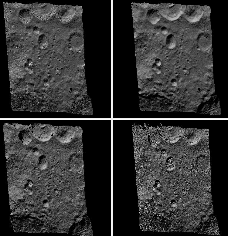
Fig. 6.1 A DEM produced (from top-left) with the asp_bm, asp_mgm,
libelas, and opencv_sgbm stereo algorithms. The libelas
algorithm is rather fast and the results are of good quality.
No mapprojection (Section 6.1.7) was used here.
The most important choice a user has to make when running ASP is the stereo algorithm to use. By default, ASP runs as if invoked with:
parallel_stereo --alignment-method affineepipolar  \
  --stereo-algorithm asp_bm --subpixel-mode 1      \
  <other options>
This invokes block-matching stereo with parabola subpixel mode, which can be fast but not of high quality. Much better results are likely produced with:
parallel_stereo                     \
  --alignment-method affineepipolar \
  --stereo-algorithm asp_mgm        \
  --subpixel-mode 9                 \
  <other options>
which uses ASP’s implementation of MGM (Section 18.2). Using
--subpixel-mode 3 will likely further improve the results, but
will be slower. For best results one can use --subpixel-mode 2,
but that is very slow. Do not use --subpixel-mode 1 with
asp_mgm/asp_sgm as that produces artifacts. See
Section 14.5 for more background on some subpixel modes.
For steep terrains it is strongly suggested to mapproject the images (Section 6.1.7).
ASP also implements local alignment, when the input images are split into tiles (with overlap) and locally aligned. This makes it possible to use third-party algorithms in addition to the ones ASP implements.
With ASP’s own MGM algorithm, local alignment can be invoked as:
parallel_stereo                     \
  --alignment-method local_epipolar \
  --stereo-algorithm asp_mgm        \
  --subpixel-mode 9                 \
  <other options>
ASP also ships with the following third-party stereo algorithms: MGM (original author implementation), OpenCV SGBM, Libelas, MSMW, MSMW2, and OpenCV BM. For more details see Section 6.1.2.2.
For example, the rather solid and reasonably fast Libelas implementation can be called as:
parallel_stereo                     \
  --alignment-method local_epipolar \
  --stereo-algorithm libelas        \
  --job-size-h 512 --job-size-w 512 \
  --sgm-collar-size 128             \
  <other options>
Above we used tiles of size 512 pixels with an extra padding of 128 pixels on
each side, for a total size of 768 pixels. Smaller tiles are easier to align
accurately, and also use less memory. The defaults in parallel_stereo are
double these values, which work well with ASP’s MGM which is more conservative
with its use of memory but can be too much for some other implementations.
It is suggested to not specify here --subpixel-mode, in which case
it will use each algorithm’s own subpixel implementation. Using
--subpixel-mode 3 will refine that result using ASP’s subpixel
implementation. Using --subpixel-mode 2 will be much slower but
likely produce even better results.
Next we will discuss more advanced parameters which rarely need to be set in practice.
6.1.2. Setting options in the stereo.default file
The parallel_stereo program can use a stereo.default file that
contains settings that affect the stereo reconstruction process. Its
contents can be altered for your needs; details are found in
Section 17. You may find it useful to save multiple
versions of the stereo.default file for various processing
needs. If you do this, be sure to specify the desired settings file by
invoking parallel_stereo with the -s option. If this option is
not given, the parallel_stereo program will search for a file
named stereo.default in the current working directory. If
parallel_stereo does not find stereo.default in the current
working directory and no file was given with the -s option,
parallel_stereo will assume default settings and continue.
An example stereo.default file is available in the top-level
directory of ASP. The actual file has a lot of comments to show you
what options and values are possible. Here is a trimmed version of the
important values in that file.
alignment-method affineepipolar
stereo-algorithm asp_bm
cost-mode 2
corr-kernel 21 21
subpixel-mode 1
subpixel-kernel 21 21
For the asp_sgm and asp_mgm algorithms, the default correlation
kernel size is 5 x 5 rather than 21 x 21.
Note that the corr-kernel option does not apply to the external
algorithms. Instead, each algorithm has its own options that need to
be set (Section 6.1.2.2).
All these options can be overridden from the command line, as described in Section 6.1.5.
6.1.2.1. Alignment method
For raw images, alignment is always necessary, as the left and right
images are from different perspectives. Several alignment methods are
supported, including local_epipolar, affineepipolar and
homography (see Section 17.1.2 for details).
Alternatively, stereo can be performed with mapprojected images
(Section 6.1.7). In effect we take a smooth
low-resolution terrain and map both the left and right raw images onto
that terrain. This automatically brings both images into the same
perspective, and as such, for mapprojected images the alignment method
is always set to none.
6.1.2.2. Stereo algorithms
ASP can invoke several algorithms for doing stereo, some internally implemented, some collected from the community, and the user can add their own algorithms as well (Section 18.8).
The list of algorithms is as follows. (See Section 18 for a full discussion.)
Algorithms implemented in ASP
- asp_bm (or specify the value ‘0’)
The ASP implementation of Block Matching. Search in the right image for the best match for a small image block in the left image. This is the fastest algorithm and works well for similar images with good texture coverage. How to set the block (kernel) size and subpixel mode is described further down. See also Section 18.2.
- asp_sgm (or specify the value ‘1’)
The ASP implementation of the Semi-Global Matching (SGM) algorithm [Hirschmuller08]. This algorithm is slow and has high memory requirements but it performs better in images with less texture. See Section 18.2 for important details on using this algorithm.
- asp_mgm (or specify the value ‘2’)
The ASP implementation of the More Global Matching (MGM) variant of the SGM algorithm [FDFM15] to reduce high frequency artifacts in the output image at the cost of increased run time. See Section 18.2 for important details on using this algorithm.
- asp_final_mgm (or specify the value ‘3’)
Use MGM on the final resolution level and SGM on preceding resolution levels. This produces a result somewhere in between the pure SGM and MGM options.
External implementations (shipped with ASP)
- mgm
The MGM implementation by its authors. See Section 18.3.
- opencv_sgbm
Semi-global block-matching algorithm from OpenCV 3. See Section 18.4.
- libelas
The LIBELAS algorithm [GRU10]. See Section 18.5.
- msmw and msmw2
Multi-Scale Multi-Window algorithm (two versions provided). See Section 18.6.
- opencv_bm
Classical block-matching algorithm from OpenCV 3. See Section 18.7.
6.1.2.3. Correlation parameters
The option corr-kernel in stereo.default define what
correlation metric (normalized cross correlation) we’ll be using and
how big the template or kernel size should be (21 pixels square). A
pixel in the left image will be matched to a pixel in the right image
by comparing the windows of this size centered at them.
Making the kernel sizes smaller, such as 15 × 15, or even 11 × 11, may improve results on more complex features, such as steep cliffs, at the expense of perhaps introducing more false matches or noise.
These options only to the algorithms implemented in ASP (those whose
name is prefixed with asp_). For externally implemented
algorithms, any options to them can be passed as part of the
stereo-algorithm field, as discussed in
Section 18.
6.1.2.4. Subpixel refinement parameters
A highly critical parameter in ASP is the value of
subpixel-mode. When set to 1, parallel_stereo performs
parabola subpixel refinement, which is very fast but not very
accurate. When set to 2, it produces very accurate results, but it is
about an order of magnitude slower. When set to 3, the accuracy and
speed will be somewhere in between the other methods.
For the algorithms not implemented in ASP itself, not specifying this field will result in each algorithm using its own subpixel mode.
The option subpixel-kernel sets the kernel size to use during
subpixel refinement (also 21 pixels square).
6.1.2.5. Search range determination
ASP will attempt to work out the minimum and maximum disparity it will search for automatically. The search range can be explicitly set with a command-line option such as:
--corr-search -80 -2 20 2
These four integers define the minimum horizontal and vertical disparity and then the maximum horizontal and vertical disparity (Section 17.2).
The search range can be tightened with the option --max-disp-spread
before full-image resolution happens.
It is suggested that these settings be used only if the run-time is high or the inputs are difficult. For more details see Section 14.4.2. The inner working of stereo correlation can be found in Section 14.
6.1.3. Performing stereo correlation
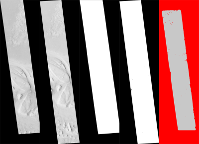
Fig. 6.2 These are the four viewable .tif files
created by the parallel_stereo program. On the left are the two aligned,
pre-processed images: (results/output-L.tif and
results/output-R.tif). The next two are mask images
(results/output-lMask.tif and results/output-rMask.tif),
which indicate which pixels in the aligned images are good to use in
stereo correlation. The image on the right is the “Good Pixel map”,
(results/output-GoodPixelMap.tif), which indicates (in gray)
which were successfully matched with the correlator, and (in red)
those that were not matched.
As already mentioned, the parallel_stereo program can be invoked for ISIS
images as:
ISIS> parallel_stereo left_image.cub right_image.cub \
          -s stereo.default results/output
For DigitalGlobe/Maxar images the cameras need to be specified separately:
parallel_stereo left.tif right.tif left.xml right.xml \
  -s stereo.default results/output
The string results/output is arbitrary, and in this case we will
simply make all outputs go to the results directory.
When parallel_stereo finishes, it will have produced a point cloud image.
Section 6.2 describes how to convert it to a digital
elevation model (DEM) or other formats.
The parallel_stereo program can be used purely for computing the
correlation (disparity) of two images, without cameras
(Section 16.17).
The quality of correlation can be evaluated with the corr_eval
program (Section 16.16).
The parallel_stereo command can also take multiple input images,
performing multi-view stereo (Section 6.4.1), though this
approach is rather discouraged as better results can be obtained with
bundle adjustment followed by pairwise stereo and merging of DEMs with
dem_mosaic (Section 16.20).
6.1.4. Running the GUI frontend
The stereo_gui program (Section 16.72) is a GUI frontend to
parallel_stereo. It is invoked with the same options as parallel_stereo
(except for the more specialized ones such as --job-size-h, etc.). It
displays the input images, and makes it possible to zoom in and select smaller
regions to run stereo on.
6.1.5. Specifying settings on the command line
All the settings given via the stereo.default file (Section 17)
can be overridden from the command line. For this add a double hyphen (--)
in front of the option’s name and set the value as in the configuration file.
For options in the stereo.default file that take multiple numbers, they must
be separated by spaces (like --corr-kernel 25 25) on the command line.
Example:
parallel_stereo E0201461.map.cub M0100115.map.cub \
   -s stereo.map --corr-search -70 -4 40 4        \
   --subpixel-mode 3 results/output
6.1.6. Stereo on multiple machines
If the input images are really large it may desirable to distribute
the work over several computing nodes. For that, the --nodes-list
option of parallel_stereo must be used. See
Section 8.19.
6.1.7. Stereo with mapprojected images
The way stereo correlation works is by matching a neighborhood of each pixel in the left image to a similar neighborhood in the right image. This matching process can fail or become unreliable if the two images are too different, which can happen for example if the perspectives of the two cameras are very different, the underlying terrain has steep portions, or because of clouds and deep shadows. This can result in large disparity search ranges, long run times, and ASP producing 3D terrains with noise or missing data.
ASP can mitigate this by mapprojecting the left and right images onto some pre-existing low-resolution smooth terrain model without holes, and using the output images to do stereo. In effect, this makes the images much more similar and more likely for stereo correlation to succeed.
In this mode, ASP does not create a terrain model from scratch, but rather uses an existing terrain model as an initial guess, and improves on it.
6.1.7.1. Choice of initial guess terrain model
For Earth, an existing terrain model can be, for example, the Copernicus 30 m DEM from:
or the NASA SRTM DEM (available on the same web site as above), GMTED2010, USGS’s NED data, or NGA’s DTED data.
The Copernicus 30 m DEM heights are relative to the EGM96 geoid.
Any such DEM must be converted using dem_geoid to WGS84 ellipsoid heights,
for any processing to be accurate. See (Section 6.1.7.2).
There exist pre-made terrain models for other planets as well, for example the Moon LRO LOLA global DEM and the Mars MGS MOLA DEM.
Check, as before, if your DEM is relative to the areoid rather than an
ellipsoid (Section 6.1.7.2). Some Mars DEMs may have an
additional 190 meter vertical offset (such as the dataset
molaMarsPlanetaryRadius0001.cub shipped with ISIS data), which can
be taken care of with image_calc (Section 16.33).
Alternatively, a low-resolution smooth DEM can be obtained by running ASP itself
(Section 6.1.7.5). In such a run, subpixel mode may be set to parabola
(subpixel-mode 1) for speed. To make it sufficiently coarse and smooth, the
resolution can be set to about 40 times coarser than either the default
point2dem (Section 16.56) resolution or the resolution of the input
images. If the resulting DEM turns out to be noisy or have holes, one could
change in point2dem the search radius factor, use hole-filling, invoke more
aggressive outlier removal, and erode pixels at the boundary (those tend to be
less reliable).
6.1.7.2. Conversion of initial guess terrain to ellipsoid heights
It is very important that your DEM be relative to a datum/ellipsoid (such as WGS84), and not to a geoid/areoid, such as EGM96 for Earth. Otherwise there will be a systematic offset of several tens of meters between the images and the DEM, which can result in artifacts in mapprojection and stereo.
A DEM relative to a geoid/areoid must be converted so that its heights are relative to an ellipsoid. This must be done for any Copernicus and SRTM DEMs. For others, consult the documentation of the source of the DEM to see this operation is needed.
The gdalwarp program in recent versions of GDAL and our own dem_geoid
tool (Section 16.19) can be used to perform the necessary conversions, if
needed. For example, with dem_geoid, one can convert EGM96 heights to WGS84
with the command:
dem_geoid --geoid egm96 --reverse-adjustment \
  dem.tif -o dem
This will create dem-adj.tif.
6.1.7.3. Hole-filling and smoothing the input DEM
It is suggested to inspect and then hole-fill the input DEM (Section 16.20.2.8 and Section 16.20.2.9).
If the input DEM has too much detail, and those features do not agree with the images mapprojected on it, this can result in artifacts in the final DEM. A blur is suggested, after the holes are filled. Example:
dem_mosaic --dem-blur-sigma 5 dem.tif -o dem_blur.tif
The amount of blur may depend on the input DEM resolution, image ground sample distance, and how misregistered the initial DEM is relative to the images. One can experiment on a clip with values of 5 and 10 for sigma, for example.
6.1.7.4. Grid size and projection
It is very important to specify the same grid size (ground sample distance,
ground resolution) and projection string when mapprojecting the images (options
--tr and --t_srs for mapproject, Section 16.41), to avoid big
search range issues later in correlation.
Normally, mapproject is rather good at auto-guessing the resolution,
so this tool can be invoked with no specification of the resolution
for the left image, then then gdalinfo can be used to find
the obtained pixel size, and that value can be used with the right image.
In the latest build ASP, these quantities can be borrowed from the first
mapprojected image with the option --ref-map (Section 16.41.2.5).
Invoking mapproject with the --query-projection option will print the
estimated ground sample distance (output pixel size) without doing the
mapprojection.
If these two images have rather different auto-determined resolutions, it is suggested that the smaller ground sample distance be used for both, or otherwise something in the middle.
Using a ground sample distance which is too different than what is appropriate can result in aliasing in mapprojected images and artifacts in stereo.
6.1.7.5. Example for ISIS images
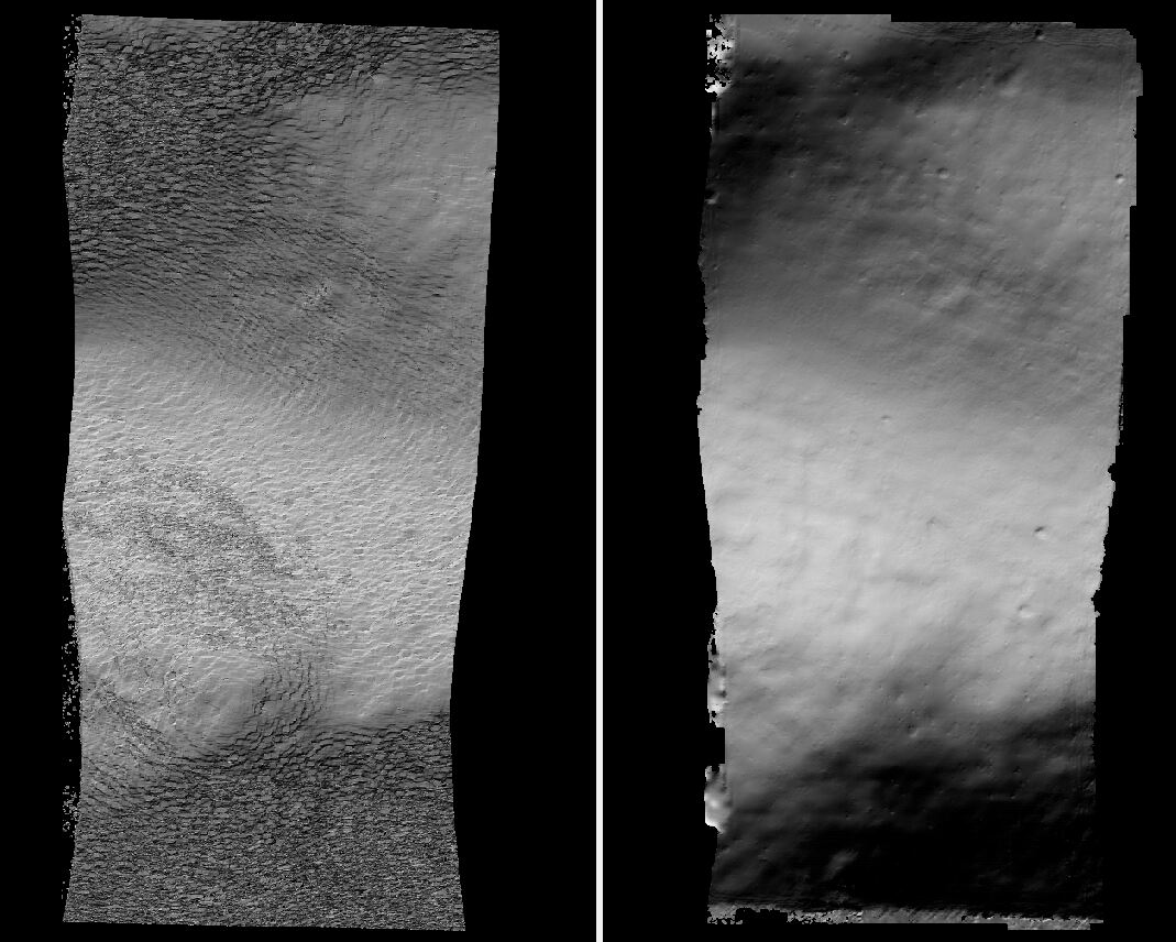
Fig. 6.3 A DEM obtained using plain stereo (left) and stereo with mapprojected images
(right). Their quality will be comparable for relatively flat terrain and the
second will be much better for rugged terrain. The right image has some
artifacts at the boundary, which could have been avoided by running without
clipping the input images or by cropping the input DEM. We used the asp_mgm
algorithm (Section 6.1).
This example illustrates how to run stereo with mapprojected images for ISIS
data. For an alternative approach using cam2map, see
Section 14.6.2.
We start with LRO NAC Lunar images M1121224102LE and M1121209902LE from ASU’s LRO NAC web site (https://wms.lroc.asu.edu/lroc/search), fetching them as:
wget http://pds.lroc.asu.edu/data/LRO-L-LROC-2-EDR-V1.0/LROLRC_0015/DATA/ESM/2013111/NAC/M1121224102LE.IMG
wget http://pds.lroc.asu.edu/data/LRO-L-LROC-2-EDR-V1.0/LROLRC_0015/DATA/ESM/2013111/NAC/M1121209902LE.IMG
We convert them to ISIS cubes using the ISIS program lronac2isis,
then we use the ISIS tools spiceinit, lronaccal, and
lrnonacecho to update the SPICE kernels and to do radiometric and
echo correction. This process is described in
Section 8.7.4. We name the two obtained .cub files
left.cub and right.cub.
Here we decided to run ASP to create the low-resolution DEM needed for mapprojection, rather than get them from an external source. For speed, we process just a small portion of the images:
parallel_stereo left.cub right.cub            \
  --left-image-crop-win 1984 11602 4000 5000  \
  --right-image-crop-win 3111 11027 4000 5000 \
  --job-size-w 1024 --job-size-h 1024         \
  --subpixel-mode 1                           \
  run_nomap/run
(the crop windows can be determined using stereo_gui,
Section 16.72.8). The input images have resolution of about 1 meter.
We create the low-resolution DEM using a resolution 40 times as coarse, with a local stereographic projection:
point2dem --stereographic --auto-proj-center --tr 40.0 \
  --search-radius-factor 5 run_nomap/run-PC.tif
Or, the projection center can be passed to point2dem such as:
point2dem --stereographic --proj-lon <lon_ctr> --proj-lat <lat_ctr>
Some experimentation with the parameters used by point2dem may be necessary
for this low-resolution DEM to be smooth enough and with no holes.
For Earth, a projection such as UTM can be used.
We used --search-radius-factor 5 to expand the DEM a
bit, to counteract future erosion at image boundary in stereo due to
the correlation kernel size. This is optional.
By calling gdalinfo -proj4, the PROJ string of the obtained DEM
can be found, which can be used in mapprojection later, and with the
resolution switched to meters from degrees (see Section 6.1.7.6
for more details).
This DEM can be hole-filled and blurred with dem_mosaic if needed
(Section 16.20.2.9), producing a DEM called
run_nomap/run-smooth.tif. Inspect the result. It should be smooth and with
no holes.
Next, we mapproject the left image onto this DEM with the mapproject program
(Section 16.41):
mapproject run_nomap/run-smooth.tif \
  left.cub left_proj.tif
The resolution of mapprojection is automatically determined, and can be later
inspected with gdalinfo (Section 16.25). The projection may be
auto-determined as well (Section 16.41.1).
It is very important to use the same resolution and projection for
mapprojecting the right image (Section 6.1.7.4), and to adjust these
below (--tr and --t_srs).
In the latest builds of ASP, mapproject can borrow the resolution and
projection for the right image from the left one that was already mapprojected,
with the --ref-map option:
mapproject                 \
  --ref-map left_proj.tif  \
  run_nomap/run-smooth.tif \
  right.cub right_proj.tif
Next, we do stereo with these mapprojected images, with the mapprojection DEM as the last argument:
parallel_stereo                \
  --stereo-algorithm asp_mgm   \
  --subpixel-mode 9            \
  --sgm-collar-size 256        \
  left_proj.tif right_proj.tif \
  left.cub right.cub           \
  run_map/run                  \
  run_nomap/run-smooth.tif
Even though we use mapprojected images, we still specified the original images
as the third and fourth arguments. That because we need the camera information
from those files. The fifth argument is the output prefix, while the sixth is
the low-resolution DEM we used for mapprojection. We have used here
--subpixel-mode 9 with the asp_mgm algorithm as this will be the final
point cloud and we want the increased accuracy.
See Section 6.1 for more details about the various speed-vs-accuracy tradeoffs for stereo.
The mapprojection DEM can be set via --dem above, in any place in the
command, rather than being the very last argument (as of build 2026/02,
Section 2.1).
Lastly, we create a DEM at 1 meter resolution with point2dem
(Section 16.56):
point2dem --stereographic \
  --auto-proj-center      \
  --tr 1.0                \
  run_map/run-PC.tif
We could have used a coarser resolution for the final DEM, such as 4 meters/pixel, since we won’t see detail at the level of 1 meter in this DEM, as the stereo process is lossy. This is explained in more detail in Section 16.56.4.
In Fig. 6.3 we show the effect of using mapprojected images on accuracy of the final DEM.
Some experimentation on a small area may be necessary to obtain the best
results. Once images are mapprojected, they can be cropped to a small
shared region using gdal_translate -projwin and then stereo with
these clips can be invoked.
We could have mapprojected the images using the ISIS tool cam2map,
as described in Section 14.6.2. The current approach
may be preferable since it allows us to choose the DEM to mapproject
onto, and it is faster, since ASP’s mapproject uses multiple
processes, while cam2map is restricted to one process and one
thread.
6.1.7.6. Example for DigitalGlobe/Maxar images
In this section we will describe how to run stereo with mapprojected images for DigitalGlobe/Maxar cameras for Earth. The same process can be used for any satellite images from any vendor (Section 6.1.7.7).
Unlike the previous section, here we will use an external DEM to
mapproject onto, rather than creating our own. We will use a variant of
NASA SRTM data with no holes. See Section 6.1.7.1 for how
to fetch such a terrain. We will name this DEM ref_dem.tif.
It is important to note that ASP expects the input low-resolution DEM
to be in reference to a datum ellipsoid, such as WGS84 or NAD83. If
the DEM is in respect to either the EGM96 or NAVD88 geoids, the ASP
tool dem_geoid can be used to convert the DEM to WGS84 or NAD83
(Section 16.19). See Section 6.1.7.2 for more
details.
Not applying this conversion might not properly negate the parallax seen between the two images, though it will not corrupt the triangulation results. In other words, sometimes one may be able to ignore the vertical datums on the input but we do not recommend doing that. Also, you should note that the geoheader attached to those types of files usually does not describe the vertical datum they used. That can only be understood by careful reading of your provider’s documents.
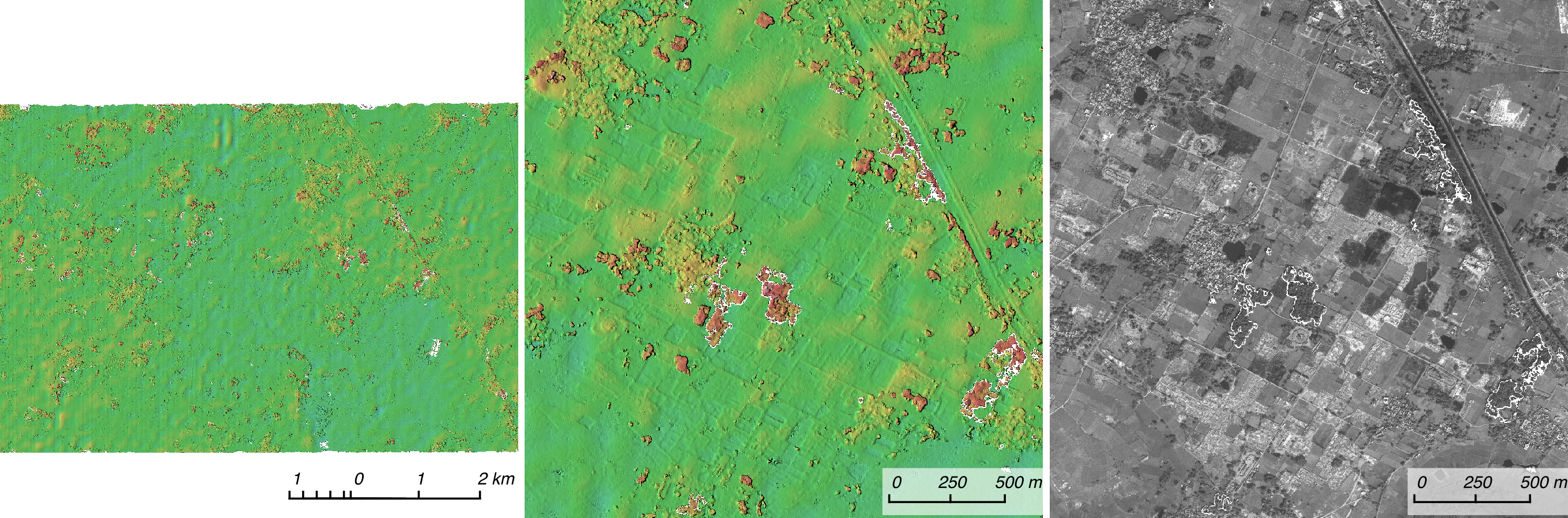
Fig. 6.4 Example colorized height map and ortho image output.
A DigitalGlobe/Maxar camera file contains both an exact (linescan) camera model and an approximate RPC camera model.
In this example, we use the exact linescan camera model for mapprojection (-t
dg). In older ASP the RPC model was used instead as it was faster (-t
rpc). Triangulation will happen either way with the exact model. Mapprojection
does not need the precise model as it can be seen as a form of
orthorectification that is undone when needed.
It is strongly suggested to use a local projection for the mapprojection, especially around poles, as there the default longitude-latitude projection is not accurate.
The same appropriately chosen resolution setting (option --tr)
must be used for both images to avoid long run-times and artifacts
(Section 6.1.7.4).
The ref_dem.tif dataset should be at a coarser resolution, such as 40 times
coarser than the input images, as discussed earlier, to ensure no
misregistration artifacts transfer over to the mapprojected images. Ensure the
input DEM is relative to an ellipsoid and not a geoid
(Section 6.1.7.2).
Fill and blur the input DEM if needed (Section 16.20.2.9).
Mapprojection commands:
proj='+proj=utm +zone=11 +datum=WGS84 +units=m +no_defs'
mapproject -t dg \
--t_srs "$proj" \
--tr 0.5 \
ref_dem.tif \
12FEB12053305-P1BS_R2C1-052783824050_01_P001.TIF \
12FEB12053305-P1BS_R2C1-052783824050_01_P001.XML \
left_mapproj.tif
mapproject -t dg \
--t_srs "$proj" \
--tr 0.5 \
ref_dem.tif \
12FEB12053341-P1BS_R2C1-052783824050_01_P001.TIF \
12FEB12053341-P1BS_R2C1-052783824050_01_P001.XML \
right_mapproj.tif
If the --t_srs option is not specified, the projection string will be read
from the low-resolution input DEM, unless the DEM is in a geographic projection,
when a projection in meters will be found (Section 16.41.1). See
Section 16.41.2.5 for how to ensure both images share the same projection
and grid size.
The zone of the UTM projection depends on the location of the images. Hence, if not relying on projection auto-determination, the zone should be set appropriately.
The complete list of options for mapproject is described in
Section 16.41.
Running parallel_stereo with these mapprojected images, and the
DEM used for mapprojection as the last argument:
parallel_stereo \
--stereo-algorithm asp_mgm \
--subpixel-mode 9 \
--alignment-method none \
--nodes-list nodes_list.txt \
left_mapproj.tif right_mapproj.tif \
12FEB12053305-P1BS_R2C1-052783824050_01_P001.XML \
12FEB12053341-P1BS_R2C1-052783824050_01_P001.XML \
dg/dg \
ref_dem.tif
See Section 6.1 for more details about the various speed-vs-accuracy tradeoffs. See Section 8.19 for running on multiple machines.
We have used alignment-method none, since the images are mapprojected onto
the same terrain with the same resolution, thus no additional alignment is
necessary. More details about how to set these and other parallel_stereo
parameters can be found in Section 6.1.2.
The mapprojection DEM can be set via --dem above, in any place in the
command, rather than being the very last argument (as of build 2026/02,
Section 2.1).
DEM creation (Section 16.56):
point2dem --tr 0.5 dg/dg-PC.tif
This DEM will inherit the projection from the mapprojected images. To auto-guess a local UTM projection, see Section 16.56.1.
6.1.7.7. Mapprojection with other camera models
Stereo with mapprojected images can be used with any camera model
supported by ASP, including RPC (Section 8.22), Pinhole
(Section 9.3), CSM (Section 8.12), OpticalBar
(Section 8.28), etc. The mapproject command needs to be invoked
with -t rpc, -t pinhole, etc., and normally it auto-detects
this option (except when a camera file has both DG and RPC
cameras).
The cameras can also be bundle-adjusted, as discussed later.
As earlier, when invoking parallel_stereo with mapprojected images, the
first two arguments should be these images, followed by the camera
models, output prefix, and the name of the DEM used for mapprojection.
The session name (-t) passed to parallel_stereo should be
rpcmaprpc, pinholemappinhole, or just rpc, pinhole,
etc. Normally this is detected and set automatically.
The stereo command with mapprojected images when the cameras are stored separately is along the lines of:
parallel_stereo \
-t rpc \
--stereo-algorithm asp_mgm \
--nodes-list nodes_list.txt \
left.map.tif right.map.tif \
left.xml right.xml \
run/run \
ref_dem.tif
or:
parallel_stereo               \
  -t pinhole                  \
  --stereo-algorithm asp_mgm  \
  --subpixel-mode 9           \
  --nodes-list nodes_list.txt \
  left.map.tif right.map.tif  \
  left.tsai right.tsai        \
  run/run                     \
  ref_dem.tif
When the cameras are embedded in the images, the command is:
parallel_stereo               \
  -t rpc                      \
  --stereo-algorithm asp_mgm  \
  --subpixel-mode 9           \
  --nodes-list nodes_list.txt \
  left.map.tif right.map.tif  \
  run/run                     \
  ref_dem.tif
If your cameras have been corrected with bundle adjustment
(Section 16.5), one should pass --bundle-adjust-prefix
to all mapproject and parallel_stereo invocations. See also
Section 16.53.14 for when alignment was used as well.
Then, point2dem can be run, as above, to create a DEM.
6.1.7.8. Reusing a run with mapprojected images
Mapprojection of input images is a preprocessing step, to help rectify them. The camera model type, bundle adjust prefix, and even camera names used in mapprojection are completely independent of the camera model type, bundle adjust prefix, and camera names used later in stereo with these mapprojected images.
Moreover, once stereo is done with one choices of these, the produced run can be reused with a whole new set of choices, with only the triangulation step needing to be redone. That because the correlation between the images is still valid when the cameras change.
This works best when the cameras do not change a lot after the initial run is made. Otherwise, it is better to redo the mapprojection and the full run from scratch.
Once such a run is done, using say the output prefix dg/dg,
parallel_stereo can be done with the option --prev-run-prefix dg/dg,
a new output prefix, and modifications to the variables above, which will
redo only the triangulation step.
Even the camera files can be changed for stereo (only with ASP 3.3.0 or later).
For example, jitter_solve (Section 16.38) can produce CSM cameras
given input cameras in Maxar / DigitalGlobe .xml files or input CSM .json files
(Section 8.12). So, if stereo was done with mapprojected images named
left_mapproj.tif and right_mapproj.tif, with cameras with names like
left.xml and right.xml, before solving for jitter, and this solver
produced cameras of the form adjusted_left.json, adjusted_right.json,
the reuse of the previous run can be done as:
parallel_stereo                          \
  left_mapproj.tif right_mapproj.tif     \
  adjusted_left.json adjusted_right.json \
  --prev-run-prefix dg/dg                \
  jitter/run                             \
  ref_dem.tif
Under the hood, this will read the metadata from the mapprojected images
(Section 16.41.3), will look up the original left.xml and
right.xml cameras, figure out what camera model was used in mapprojection
will undo the mapprojection with this data, and then will do the triangulation
with the new cameras.
It is very important that --bundle-adjust-prefix needs to be used or not
depending on the circumstances. For example, jitter-solved cameras already
incorporate any prior bundle adjustment that jitter_solve was passed on
input, so it was not specified in the above invocation, and in fact the results
would be wrong if it was specified.
An example without mapprojected images is shown in Section 8.31.11.
6.1.7.9. Stereo with ortho-ready images
Some vendors offer orthoimages that have been projected onto surfaces of constant height above a datum. Examples are Maxar’s OR2A product and the Airbus Pleiades ortho product. These can be processed with ASP after some preparation.
The orthoimages may have different pixel sizes (as read with gdalinfo,
Section 16.25). The coarser one must be regridded to the pixel size of
the finer one, with a command such as:
gdalwarp -r cubicspline -overwrite -tr 0.4 0.4 \
  ortho.tif ortho_regrid.tif
The orthoimages must have the same projection, in units of meters (such as UTM).
If these are different, the desired projection string can be added to the
gdalwarp command above via the option -t_srs. If desired to also clip
both images to a region, add the option -te <xmin> <ymin> <xmax> <ymax>.
The stereo command is:
parallel_stereo                    \
  -t rpc                           \
  --stereo-algorithm asp_mgm       \
  --ortho-heights 23.5 27.6        \
  left_regrid.tif right_regrid.tif \
  left.xml right.xml               \
  run/run
The values passed in via --ortho-heights are the heights above the
datum that were used to project the images. The datum is read from the
geoheader of the images.
For Maxar OR2A data (as evidenced by the ORStandard2A tag in the XML camera
files), the option --ortho-heights need not be set, as the entries will be
auto-populated from the <TERRAINHAE> field in the camera files.
The option --ortho-heights, if set, takes priority over fields in those
camera files.
For Pleiades data, the needed values need to be looked up as described in Section 8.24.5, and then set as above.
All products we encountered (both Maxar and Airbus Pleiades) employed the RPC
camera model. If that model is of a different type, adjust the -t option
above (Section 16.51.8).
After stereo, point2dem (Section 16.56) is run as usual. It is
suggested to inspect the triangulation error created by that program, and to
compare with a prior terrain, such as in Section 6.1.7.1.
6.1.8. Diagnosing problems
Once invoked, parallel_stereo proceeds through several stages that are
detailed in Section 16.51.7. Intermediate and final output
files are generated as it goes. See Section 19, page for
a comprehensive listing. Many of these files are useful for diagnosing
and debugging problems. For example, as Fig. 6.2
shows, a quick look at some of the TIFF files in the results/
directory provides some insight into the process.
Perhaps the most accessible file for assessing the quality of your
results is the good pixel image (results/output-GoodPixelMap.tif).
If this file shows mostly good, gray pixels in the overlap area
(the area that is white in both the results/output-lMask.tif
and results/output-rMask.tif files), then your results are just
fine. If the good pixel image shows lots of failed data, signified
by red pixels in the overlap area, then you need to go back and
tune your stereo.default file until your results improve. This
might be a good time to make a copy of stereo.default as you
tune the parameters to improve the results.
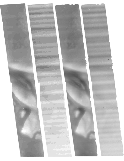
Fig. 6.5 Disparity images produced using the
disparitydebug tool. The two images on the left are the
results/output-D-H.tif and results/output-D-V.tif files,
which are normalized horizontal and vertical disparity components
produced by the disparity map initialization phase. The two images on
the right are results/output-F-H.tif and
results/output-F-V.tif, which are the final filtered,
sub-pixel-refined disparity maps that are fed into the Triangulation
phase to build the point cloud image. Since these MOC images were
acquired by rolling the spacecraft across-track, most of the
disparity that represents topography is present in the horizontal
disparity map. The vertical disparity map shows disparity due to
“wash-boarding”, which is not due to topography but because of spacecraft
movement. Note however that the horizontal and vertical disparity
images are normalized independently. Although both have the same
range of gray values from white to black, they represent
significantly different absolute ranges of disparity.
Whenever parallel_stereo, point2dem, and other executables are run, they
create log files in given tool’s results directory, containing a copy of the
configuration file, the command that was run, your system settings, and tool’s
console output. This will help track what was performed so that others in the
future can recreate your work.
Another handy debugging tool is the disparitydebug program
(Section 16.23), which allows you to generate viewable
versions of the intermediate results from the stereo correlation
algorithm. disparitydebug converts information in the disparity
image files into two TIFF images that contain horizontal and vertical
components of the disparity (i.e. matching offsets for each pixel in
the horizontal and vertical directions). There are actually three
flavors of disparity map: the -D.tif, the -RD.tif, and
-F.tif. You can run disparitydebug on any of them. Each shows
the disparity map at the different stages of processing.
disparitydebug results/output-F.tif
If the output H and V files from disparitydebug look good, then the
point cloud image is most likely ready for post-processing. You can
proceed to make a mesh or a DEM by processing results/output-PC.tif
using the point2mesh or point2dem tools, respectively.
Fig. 6.5 shows the outputs of disparitydebug.
If the input images are mapprojected (georeferenced) and the alignment
method is none, all images output by stereo are georeferenced as
well, such as GoodPixelMap, D_sub, disparity, etc. As such, all these
data can be overlaid in stereo_gui. disparitydebug also
preserves any georeference.
6.1.9. Dealing with long run-times and failures
If stereo_corr takes unreasonably long, it may have encountered a portion of
the image where, due to noise (such as clouds, shadows, etc.) the determined
search range is much larger than what it should be. The search range is
displayed in a terminal and saved to stereo_corr log files
(Section 19.8). A width and height over 100 pixels is generally too
large.
In this case it is suggested to mapproject the images (Section 6.1.7). This will make the images more similar and reduce the search range.
A few other strategies, with or without mapprojected images, are as follows.
If running on multiple machines, ensure the --nodes-list option is used
(Section 8.19).
With the default block-matching algorithm, --stereo-algorithm
asp_bm, the option --corr-timeout integer can be used to limit
how long each 1024 × 1024 pixel tile can take. A good value here
could be 300 (seconds) or more if your terrain is expected to have
large height variations.
With the asp_sgm or asp_mgm algorithms, set a value
for --corr-memory-limit-mb (Section 18.2) for the number
of megabytes of memory to use for each correlation process.
This needs to take into account how much memory is available
and how many processes are running in parallel per node.
To remove outliers one can tighten --outlier-removal-params
(Section 17), or mapproject the images (Section 6.1.7).
A smaller manual search range can be specified (Section 6.1.2.5).
In particular, with mapprojected images, the option --max-disp-spread
can be very useful (Section 17.2).
If a run failed partially during correlation, it can be resumed with the
parallel_stereo option --resume-at-corr (Section 16.51). A
ran can be started at the triangulation stage after making changes to the
cameras while reusing a previous run with the option --prev-run-prefix.
If a run failed due to running out of memory with
asp_mgm/asp_sgm, also consider lowering the value of
--processes.
See also Section 5.4 with considers the situation that clouds are present in the input images. The suggestions there may apply in other contexts as well.
On Linux, the parallel_stereo program writes in each output tile
location a file of the form:
<tile prefix>-<program name>-resource-usage.txt
having the elapsed time and memory usage, as output by /usr/bin/time.
This can guide tuning of parameters to reduce resource usage.
6.1.10. Correcting camera positions and orientations
The bundle_adjust program (Section 16.5) can be used to
adjust the camera positions and orientations before running
stereo. These adjustments makes the cameras self-consistent, but not
consistent with the ground.
A stereo terrain created with bundle-adjusted cameras can be aligned
to an existing reference using pc_align
(Section 6.1.11). The same alignment transform can be
applied to the bundle-adjusted cameras (Section 16.53.14).
6.1.11. Alignment to point clouds from a different source
Often the 3D terrain models output by parallel_stereo (point
clouds and DEMs) can be intrinsically quite accurate yet their actual
position on the planet may be off by several meters or several
kilometers, depending on the spacecraft. This can result from small
errors in the position and orientation of the satellite cameras taking
the pictures.
Such errors can be corrected in advance using bundle adjustment, as
described in the previous section. That requires using ground control
points, that may not be easy to collect. Alternatively, the images and
cameras can be used as they are, and the absolute position of the output
point clouds can be corrected in post-processing. For that, ASP provides
a tool named pc_align (Section 16.53).
This program aligns a 3D terrain to a much more accurately positioned (if
potentially sparser) dataset. Such datasets can be made up of GPS measurements
(in the case of Earth), or from laser altimetry instruments on satellites, such
as ICESat/GLASS for Earth, LRO/LOLA on the Moon, and MGS/MOLA on Mars
(Section 19.12.4). Under the hood, pc_align uses the Iterative Closest
Point algorithm (ICP) (both the point-to-plane and point-to-point flavors are
supported, and with point-to-point ICP it is also possible to solve for a scale
change).
The pc_align tool requires another input, an a priori guess for the
maximum displacement we expect to see as result of alignment, i.e., by
how much the points are allowed to move when the alignment transform is
applied. If not known, a large (but not unreasonably so) number can be
specified. It is used to remove most of the points in the source
(movable) point cloud which have no chance of having a corresponding
point in the reference (fixed) point cloud.
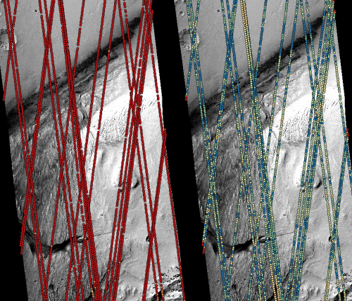
Fig. 6.6 Example of using pc_align to align a DEM obtained using stereo
from CTX images to a set of MOLA tracks. The MOLA points are colored
by the offset error initially (left) and after pc align was applied
(right) to the terrain model. The red dots indicate more than 100 m
of error and blue less than 5 m. The pc_align algorithm
determined that by moving the terrain model approximately 40 m south,
70 m west, and 175 m vertically, goodness of fit between MOLA and the
CTX model was increased substantially.
Here is an example. Recall that the denser reference cloud is specified first,
the sparser source cloud to be aligned is specified second, and that this
program is very sensitive to the value of --max-displacement
(Section 16.53.2):
pc_align --max-displacement 200           \
  --datum MOLA                            \
  --save-transformed-source-points        \
  --save-inv-transformed-reference-points \
  --csv-format '1:lon 2:lat 3:radius_m'   \
  stereo-PC.tif mola.csv                  \
  -o align/run
The cloud mola.csv will be transformed to the coordinate system
of stereo-PC.tif and saved as run/run-trans_source.csv.
The cloud stereo-PC.tif will be transformed to to the coordinate system of
mola.csv and saved as align/run-trans_reference.tif. It can
then be gridded with point2dem (Section 16.56) and compared to
mola.csv using geodiff (Section 16.26).
Validation and error metrics are discussed in Section 16.53.10 and Section 16.53.9.
It is important to note here that there are two widely used Mars datums, and if
your CSV file has, unlike above, the heights relative to a datum, the correct
datum name must be specified via --datum. Section 16.56.3 talks in more
detail about the Mars datums.
See an illustration in Fig. 6.6.
An alignment transform can be applied to cameras models (Section 16.53.14). The complete documentation for this program is in Section 16.53.
6.1.12. Validation of alignment
The pc_align program saves some error report files in the output directory
(Section 16.53.9). The produced aligned cloud can be compared to the
cloud it was aligned to.
Section 16.53.10 has more details on this, including how to use
the geodiff program (Section 16.26) to take the difference between clouds,
which can then be colorized.
6.1.13. Alignment and orthoimages
After ASP has created a DEM, and the left and right images are mapprojected to
it, they are often shifted in respect to each other. That is due to the errors
in camera positions. To rectify this, one has to run bundle_adjust
(Section 16.5) first, then rerun stereo, DEM creation, followed by
mapprojection onto the new DEM. For each of these, the bundle-adjusted cameras must
be passed in via --bundle-adjust-prefix.
Note that this approach will create self-consistent outputs, but which are not necessarily aligned with pre-existing ground truth. That can be accomplished as follows.
First, need to align the DEM to the ground truth with pc_align
(Section 16.53). Then, invoke bundle_adjust on the two input images and
cameras, while passing to it the transform obtained from pc_align via the
--initial-transform option. This will move the cameras to be consistent
with the ground truth. Then one can mapproject with the updated cameras.
This approach is described in detail in Section 16.53.14.
If the alignment is applied not to a DEM, but to the triangulated point cloud
produced by stereo, one can use point2dem with the --orthoimage option,
with the point cloud after alignment and the L image before alignment.
See Section 16.56 for the description of this option and an example.
If the alignment was done with the DEM produced from a triangulated point
cloud, it can be applied with pc_align to the point cloud and then
continue as above.
6.2. Manipulating the results
When parallel_stereo finishes, it will have produced a point cloud image,
with a name like results/output-PC.tif (Section 19), which can be
used to create many kinds of data products, such as DEMs and orthoimages
(Section 16.56), textured meshes (Section 16.58), LAS files
(Section 16.57), colormaps (Section 16.14), hillshaded images
(Section 6.2.6), etc.
Produced DEMs can also be mosaicked (Section 16.20), subtracted from other DEMs or CSV files (Section 16.26), aligned to a reference (Section 6.1.11), etc.
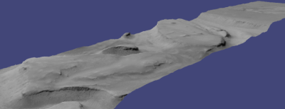
Fig. 6.7 A visualization of a mesh.
6.2.1. Building a 3D mesh model
The point2mesh command (Section 16.58) can create a 3D textured mesh
in the plain text .obj format that can be opened in a mesh viewer such as
MeshLab. The point2mesh program takes the point cloud file and the left
normalized image as inputs:
point2mesh --center results/output-PC.tif results/output-L.tif
The option --center shifts the points towards the origin, as otherwise the
mesh may have rendering artifacts because of the large values of the vertices.
Each mesh will have its own shift, however, so this option will result in meshes
that are not aligned with each other.
An example visualization is shown in Fig. 6.7.
If you already have a DEM and an ortho image (Section 6.2.2), they can be used to build a mesh as well, in the same way as done above:
point2mesh --center results/output-DEM.tif results/output-DRG.tif
6.2.2. Building a digital elevation model and ortho image
Running the point2dem program (Section 16.56):
point2dem --auto-proj-center results/output-PC.tif
will creates a Digital Elevation Model (DEM) named results/output-DEM.tif.
The default projection will be in units of meters. See Section 16.56.1
for how to set a projection or how auto-guessing it works. The planetary
body is usually auto-guessed as well, or can be set explicitly with the
an option such as -r mars.
The DEM can be transformed into a hill-shaded image for visualization
(Section 6.2.6). The DEM can be examined in stereo_gui, as:
stereo_gui --hillshade results/output-DEM.tif
The point2dem program can also be used to orthoproject raw satellite
images onto the DEM. To do this, invoke point2dem just as before,
but add the --orthoimage option and specify the use of the left
image file as the texture file to use for the projection:
point2dem --auto-proj-center \
  results/output-PC.tif      \
  --orthoimage results/output-L.tif
The texture file L.tif must always be specified after the point
cloud file PC.tif in this command.
This produces results/output-DRG.tif, which can be visualized in
stereo_gui. See Fig. 6.8 on the right for the
output image.
To fill in any holes in the obtained orthoimage, one can invoke it with
a larger value of the grid size (the --tr option) and/or with a
variation of the options:
--no-dem --orthoimage-hole-fill-len 100 --search-radius-factor 2
The point2dem program is also able to accept output projection
options the same way as the tools in GDAL. Well-known EPSG, IAU2000
projections, and custom PROJ or WKT strings can applied with the target
spatial reference set flag, --t_srs. If the target spatial reference
flag is applied with any of the reference spheroid options, the
reference spheroid option will overwrite the datum defined in the target
spatial reference set.
The following two examples produce the same output. However, the last one will also show correctly the name of the datum in the geoheader, not just the values of its axes.
point2dem --t_srs "+proj=longlat +a=3396190 +b=3376200"          \
   results/output-PC.tif

point2dem --t_srs                                                \
  'GEOGCS["Geographic Coordinate System",
     DATUM["D_Mars_2000",
     SPHEROID["Mars_2000_IAU_IAG",3396190,169.894447223611]],
     PRIMEM["Greenwich",0],
     UNIT["degree",0.0174532925199433]]'                         \
  results/output-PC.tif
The point2dem program can be used in many different ways. The
complete documentation is in Section 16.56.
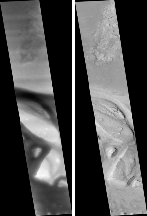
Fig. 6.8 The image on the left is a normalized DEM (generated using
the point2dem option -n), which shows low terrain
values as black and high terrain values as white. The image on the
right is the left input image projected onto the DEM (created using
the --orthoimage option to point2dem).
6.2.3. Orthorectification of an image from a different source
If you have already obtained a DEM, using ASP or some other approach,
and have an image and camera pair which you would like to overlay on top
of this terrain, use the mapproject tool (Section 16.41).
6.2.4. Creating DEMs relative to the geoid/areoid
The DEMs generated using point2dem are in reference to a datum
ellipsoid. If desired, the dem_geoid (Section 16.19)
program can be used to convert
this DEM to be relative to a geoid/areoid on Earth/Mars respectively.
Example usage:
dem_geoid results/output-DEM.tif
6.2.5. Converting to the LAS format
If it is desired to use the parallel_stereo generated point cloud outside of
ASP, it can be converted to the LAS file format, which is a public file
format for the interchange of 3-dimensional point cloud data. The tool
point2las can be used for that purpose (Section 16.57). Example usage:
point2las --compressed -r Earth results/output-PC.tif
6.2.6. Generating color hillshade maps
Once you have generated a DEM file, you can use the colormap
(Section 16.14) and hillshade (Section 16.28) programs to create
colorized and/or shaded relief images.
To create a colorized version of the DEM, you need only specify the DEM file to use. The colormap is applied to the full range of the DEM, which is computed automatically. Alternatively you can specify your own min and max range for the color map.
colormap results/output-DEM.tif -o colorized.tif
See Section 16.14 for available colormap styles and illustrations for how they appear.
To create a hillshade of the DEM, specify the DEM file to use. You can
control the azimuth and elevation of the light source using the -a
and -e options.
hillshade results/output-DEM.tif -o shaded.tif -e 25 -a 300
To create a colorized version of the shaded relief file, specify the DEM and the shaded relief file that should be used:
colormap results/output-DEM.tif -s shaded.tif -o color-shaded.tif
This program can also create the hillshaded file first, and then apply it, if
invoked with the option --hillshade.
See Fig. 6.9 showing the images obtained with these commands.
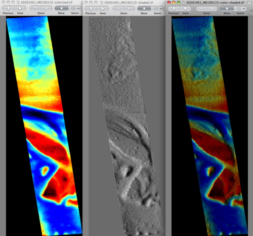
Fig. 6.9 The colorized DEM, the shaded relief image, and the colorized hillshade.
6.2.7. Cloud-Optimized GeoTIFF
ASP supports writing cloud-optimized GeoTIFFs (COG) with the --cog option
for point2dem, mapproject, image_mosaic, dem_mosaic,
geodiff, image_calc, hillshade, and colormap.
This creates files with 512 x 512 tiles, internal overviews (pyramids), and optimized compression for efficient streaming from cloud storage.
Use gdalinfo (Section 16.25) to check if an output file is a COG.
6.3. Visualizing the results
The stereo_gui program (Section 16.72) is a very versatile
viewer that can overlay hillshaded DEMs, orthoimages, interest point matches,
ASP’s report files in CSV format, polygons, etc.
6.3.1. Diagnostic plots and reports with asp_plot
The asp_plot Python package can be used to generate diagnostic plots and comprehensive PDF reports from ASP outputs. It provides visualization of stereo DEMs (hillshades, colormaps, difference maps), bundle adjustment residuals, interest point matches, map-projected image overlays, CSM camera model comparisons, and stereo geometry. For Earth-based datasets, it also supports comparison against ICESat-2 altimetry data via SlideRule.
The asp_plot package supports processing outputs from many sensors,
including WorldView, LRO NAC, etc. (Section 8).
asp_plot is available via conda and pip:
conda install -c conda-forge asp_plot
or:
pip install asp_plot
For full documentation, including installation, CLI usage, example notebooks, and example reports, see the asp_plot documentation.
6.3.2. Building overlays for Moon and Mars mode in Google Earth
Sometimes it may be convenient to see how the DEMs and orthoimages
generated by ASP look on top of existing images in Google Earth. ASP
provides a tool named image2qtree for that purpose. It creates
multi-resolution image tiles and a metadata tree in KML format that can
be loaded into Google Earth from your local hard drive or streamed from
a remote server over the Internet.
The image2qtree program can only be used on 8-bit image files with
georeferencing information (e.g. grayscale or RGB GeoTIFF images). In
this example, it can be used to process
results/output-DEM-normalized.tif, results/output-DRG.tif,
shaded.tif,colorized.tif, and shaded-colorized.tif.These images were generated respectively by using point2dem with the
-n option creating a normalized DEM, the --orthoimage option to
point2dem which projects the left image onto the DEM, and the images
created earlier with colormap.
Here’s an example of how to invoke this program:
image2qtree shaded-colorized.tif -m kml --draw-order 100
Fig. 6.10 shows the obtained KML files in Google Earth.
The complete documentation is in Section 16.31.
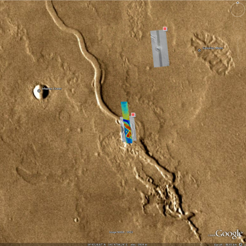
Fig. 6.10 The colorized hillshade DEM as a KML overlay.
6.3.3. Using DERT to visualize terrain models
The open source Desktop Exploration of Remote Terrain (DERT) software tool can be used to explore large digital terrain models, like those created by the Ames Stereo Pipeline. For more information, visit https://github.com/nasa/DERT.
6.3.4. Using Blender to visualize meshes
The point2mesh program will create .obj and .mtl files
that you can import directly into Blender (https://www.blender.org/).
Remember that .obj files don’t particularly have a way to
specify ‘units’ but the ‘units’ of an .obj file written out by ASP
are going to be ‘meters.’ If you open a large .obj model created by
ASP (like HiRISE), you’ll need to remember to move the default
viewpoint away from the origin, and extend the clipping distance to a
few thousand (which will be a few kilometers), otherwise it may
‘appear’ that the model hasn’t loaded (because
your viewpoint is inside of it, and you can’t see far enough).
The default step size for point2mesh is 10, which only samples
every 10th point, so you may want to read the documentation which
talks more about the -s argument to point2mesh. Depending on how
big your model is, even that might be too small, and I’d be very
cautious about using -s 1 on a HiRISE model that isn’t cropped
somehow first.
You can also use point2mesh to pull off this trick with
terrain models you’ve already made (maybe with SOCET or something
else). Our point2mesh program certainly knows how to read
our ASP *-PC.tif files, but it can also read GeoTIFFs. So if
you have a DEM as a GeoTIFF, or an ISIS cube which is a terrain
model (you can use gdal_translate to convert them to GeoTIFFs),
then you can run point2mesh on them to get .obj and
.mtl files.
6.3.5. Using MeshLab to visualize meshes
MeshLab is another program that can view meshes in
.obj files. It can be downloaded from:
https://github.com/cnr-isti-vclab/meshlab/releases
and can be installed and run in user’s directory without needing administrative privileges.
6.3.6. Using QGIS to visualize terrain models
The free and open source geographic information system QGIS (https://qgis.org) as of version 3.0 has a 3D Map View feature that can be used to easily visualize perspective views of terrain models.
After you use point2dem to create a terrain model (the
*-DEM.tif file), or both the terrain model and an ortho image
via --orthoimage (the *-DRG.tif file), those files can be
loaded as raster data files, and the ‘New 3D Map View’ under the
View menu will create a new window, and by clicking on the wrench
icon, you can set the DEM file as the terrain source, and are able
to move around a perspective view of your terrain.
6.4. Use of existing terrain data
ASP’s tools can incorporate prior ground data, such as DEMs, lidar point clouds, or GCP files (Section 16.5.9).
ASP assumes such data is well-aligned with the input images and cameras. To perform such alignment, one may first run bundle adjustment (Section 16.5), followed by stereo (Section 16.51), DEM creation (Section 16.56), alignment of DEM to existing terrain (Section 6.1.11), and then the aligment can be applied to the bundle-adjusted cameras (Section 16.53.14).
Any input terrain is assumed to be relative to a datum ellipsoid,
otherwise it should be converted with dem_geoid (Section 6.1.7.2).
This applies, in particular, to OpenTopography DEMs (Section 6.1.7.1).
These are the various approaches of integrating well-aligned prior terrain data.
Bundle adjustment can be performed with a terrain constraint. If the terrain is a DEM, use the
--heights-from-demoption (Section 12.2.1.3). This also works for a rather dense point cloud in various formats, after gridding it withpoint2dem.The
jitter_solveprogram (Section 16.38) can be called in the same way with the option--heights-from-dem.For sparse point clouds or DEM data, the
bundle_adjustoption named--reference-terraincan be invoked (Section 12.2.1.4). This one is harder to use as it takes as input stereo disparities.The
jitter_solveprogram also has the option--reference-terrain. This one is easier to use than the analogousbundle_adjustoption, as the unaligning of the disparity is done for the user on the fly (Section 16.38.16).Low-resolution stereo disparity can be initialized from a DEM, with the option
--corr-seed-mode 2(Section 14.3.2).Stereo can be run with mapprojected images. The DEM for mapprojection can be external, or from a previous stereo run (Section 6.1.7).
GCP files (Section 16.5.9) can be incorporated into bundle adjustment and jitter solving. These can also be used for aligment with
pc_align(as the source cloud).Given a prior DEM and an ASP-produced DEM, ASP can create dense correspondences between hillshaded versions of these, that can be passed to the
dem2gcpprogram (Section 16.18) to produce dense GCP. This can help correct warping in the ASP-produced DEM, by either solving for lens distortion or jitter.
6.4.1. Multi-view stereo
ASP supports multi-view stereo at the triangulation stage. This mode is discouraged.
See instead Section 9.3.5 for an approach based on pairwise stereo.
If using this multiview stereo mode (not suggested), the first image is set as reference, disparities are computed from it to all the other images, and then joint triangulation is performed [SSL01]. A single point cloud is generated with one 3D point for each pixel in the first image. The inputs to multi-view stereo and its output point cloud are handled in the same way as for two-view stereo (e.g., inputs can be mapprojected, the output can be converted to a DEM, etc.).
It is suggested that images be bundle-adjusted (Section 12.2) before running multi-view stereo.
Example (for ISIS with three images):
parallel_stereo file1.cub file2.cub file3.cub results/run
Example (for DigitalGlobe/Maxar data with three mapprojected images):
parallel_stereo file1.tif file2.tif file3.tif \
  file1.xml file2.xml file3.xml               \
  results/run input-DEM.tif
For a sequence of images, multi-view stereo can be run several times
with each image as a reference, and the obtained point clouds combined
into a single DEM using point2dem (Section 16.56).
The ray intersection error, the fourth band in the point cloud file, is computed as twice the mean of distances from the optimally computed intersection point to the individual rays. For two rays, this agrees with the intersection error for two-view stereo which is defined as the minimal distance between rays. For multi-view stereo this error is much less amenable to interpretation than for two-view stereo, since the number of valid rays corresponding to a given feature can vary across the image, which results in discontinuities in the intersection error.