16.60. sat_sim

The sat_sim satellite simulator program models a satellite traveling around a planet and taking pictures. It can either create camera models (Pinhole or Linescan), or read them from disk. In either case it creates synthetic images for the given cameras. This tool can model camera jitter.

The inputs are a DEM and georeferenced image (ortho image) of the area of interest. See Section 16.60.10 for how to create such inputs.

If the input cameras are not specified, the orbit is determined by given endpoints. It is represented as a straight edge in the projected coordinate system of the DEM, which results in an arc around the planet.

The images are created with bicubic interpolation in the ortho image and are saved with float pixels. Missing pixels will have nodata values.

If the cameras are created from scratch, the camera view can follow a custom path on the surface with varying orientation (Section 16.60.3), or the cameras can have a fixed orientation, without (Section 16.60.4) and with (Section 16.60.5) ground constraints.

The cameras are assumed to be of Pinhole (Frame) type by default, and are saved as .tsai files (Section 20.1). The option --save-as-csm can be used to save the cameras in CSM format (Section 8.12). Linescan cameras are supported as well (Section 16.60.7). Lens distortion is not modeled.

Several use cases are below.

16.60.1. Use given cameras

sat_sim --dem dem.tif --ortho ortho.tif          \
--camera-list camera_list.txt                    \
--image-size 800 600                             \
-o run/run

The camera names in the list should be one per line. The produced image names will be created from camera names by keeping the filename (without directory name) and replacing the extension with .tif. They will start with specified output prefix. Hence, if the input camera is path/to/camera.tsai, the output image will be run/run-camera.tif.

The value of --image-size should be chosen so that the ground sample distance of the produced images is close to the one of the input ortho image.

To see how a created image projects onto the ground, run mapproject (Section 16.40) as:

mapproject dem.tif run/run-camera.tif path/to/camera.tsai \
  camera.map.tif

The images can be overlaid in stereo_gui (Section 16.67).

16.60.2. Generate nadir-pointing cameras

sat_sim --dem dem.tif --ortho ortho.tif              \
--first 397.1 400.7 450000 --last 397.1 500.7 450000 \
--num 5                                              \
--focal-length 450000 --optical-center 500 500       \
--image-size 1000 1000                               \
-o run/run

See Section 16.60.4 for how to apply a custom rotation to the cameras.

The first and last cameras will be located as specified by --first and --last (Section 16.60.12). See also --frame-rate.

In this example, the camera is 450,000 m above the ground and the focal length is 450,000 pixels. If the magnitude of DEM heights is within several hundred meters, this will result in the ground sample distance being around 1 meter per pixel.

The produced image and camera names will be along the lines of:

run/run-10000.tif
run/run-10000.tsai

The resulting cameras will point in a direction perpendicular to the orbit trajectory. They will point precisely to the planet center only if the orbit endpoints are at the same height and the datum is spherical.

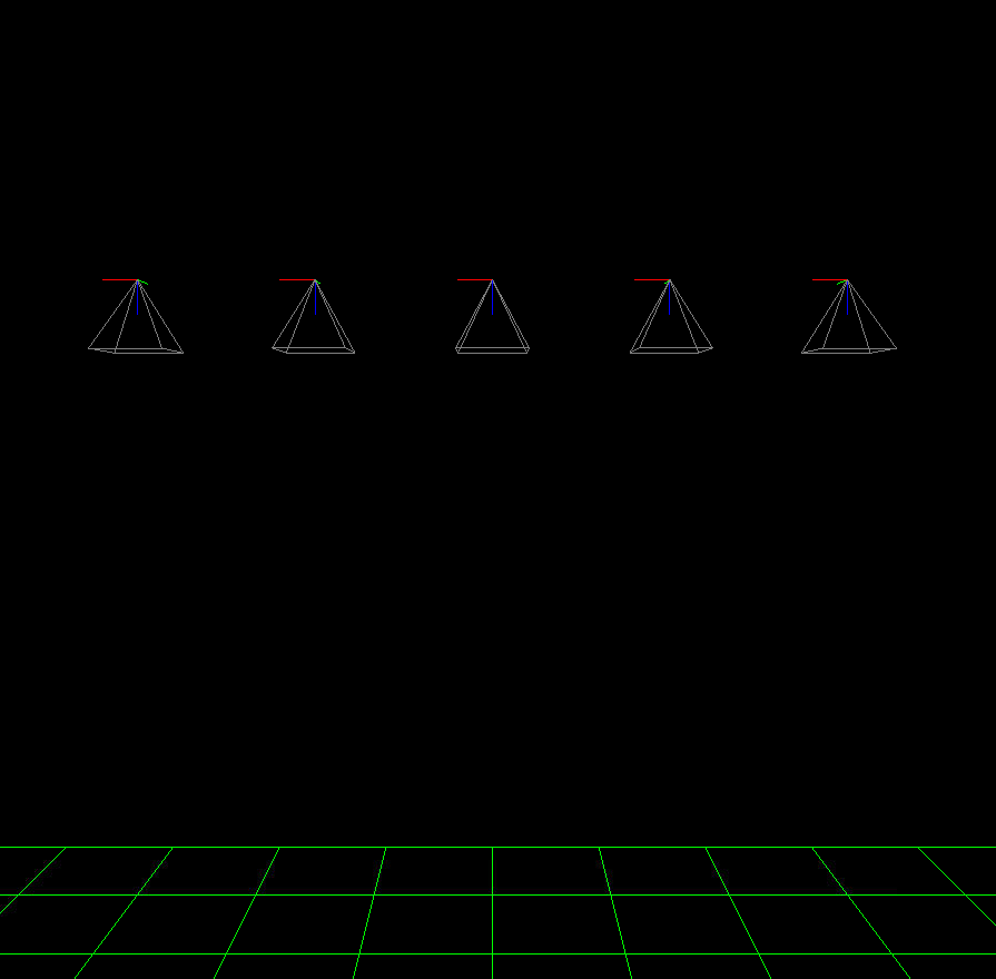
Fig. 16.24 Illustration of sat_sim creating nadir-looking cameras. See Section 16.43 for how to visualize the roll, pitch, and yaw angles of the cameras with orbit_plot.py.

16.60.3. Follow custom ground path with varying orientation

Given two locations on the DEM, each specified by the column and row of DEM pixel, to ensure that the center of the camera footprint travels along the straight edge (in DEM pixel coordinates) between these, use options as:

--first-ground-pos 484.3 510.7 \
--last-ground-pos  332.5 893.6

This will result in the camera orientation changing gradually to keep the desired view.

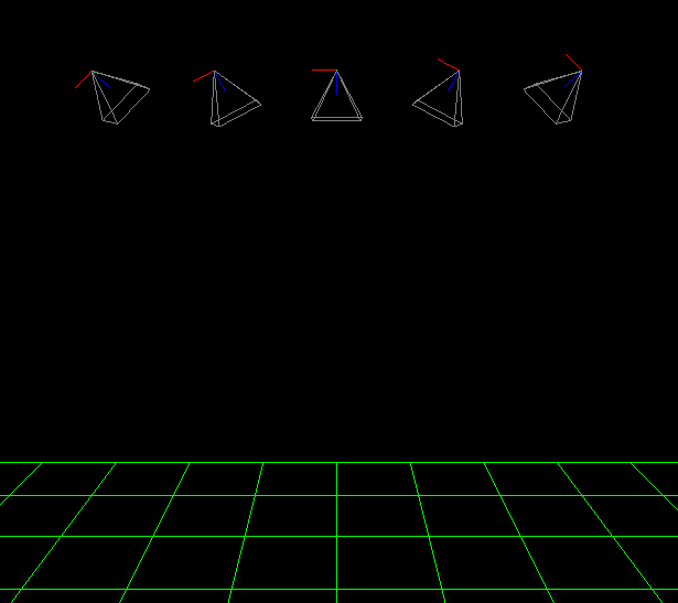
Fig. 16.25 An example of several generated cameras looking at the same ground point. Plotted with sfm_view (Section 16.63).

16.60.4. Fixed camera orientation

When custom cameras are created (not read from disk), and unless the --first-ground-pos and --last-ground-pos options are specified, the cameras will look straight down (nadir, perpendicular to along and across track directions).

If desired to have a custom orientation, use the --roll, --pitch and --yaw options (measured in degrees, all three must be specified). See Section 16.60.8 for how these angles are defined.

Example invocation:

sat_sim --dem dem.tif --ortho ortho.tif              \
--first 397.1 400.7 450000 --last 397.1 500.7 450000 \
--num 5                                              \
--roll 0 --pitch 25 --yaw 0                          \
--focal-length 450000 --optical-center 500 500       \
--image-size 1000 1000                               \
-o run/run

See Section 16.43 for how to visualize the roll, pitch, and yaw angles of the cameras with orbit_plot.py.

16.60.5. Pose and ground constraints

Given an orbital trajectory, a path on the ground, and a desired fixed camera orientation (roll, pitch, yaw), this tool can find the correct endpoints along the satellite orbit, then use those to generate the cameras (positioned between those endpoints), with the center of the camera ground footprint following the desired ground path. Example:

sat_sim --dem dem.tif --ortho ortho.tif                 \
  --first 397.1 400.7 450000 --last 397.1 500.7 450000  \
  --first-ground-pos 397.1 400.7                        \
  --last-ground-pos  397.1 500.7                        \
  --roll 0 --pitch 25 --yaw 0                           \
  --num 5                                               \
  --focal-length 450000 --optical-center 500 500        \
  --image-size 1000 1000                                \
  -o run/run

Here, unlike in Section 16.60.2, we will use --first and --last only to identify the orbit. The endpoints to use on it will be found given that we have to satisfy the orientation constraints in --roll, --pitch, --yaw and the ground path constraints in --first-ground-pos and --last-ground-pos.

Unlike in Section 16.60.3, the camera orientations will not change.

It is not important to know very accurately the values of --first-ground-pos and --last-ground-pos. The trajectory of the camera center ground footprint will be computed, points on it closest to these two ground coordinates will be found, which in turn will be used to find the orbital segment endpoints.

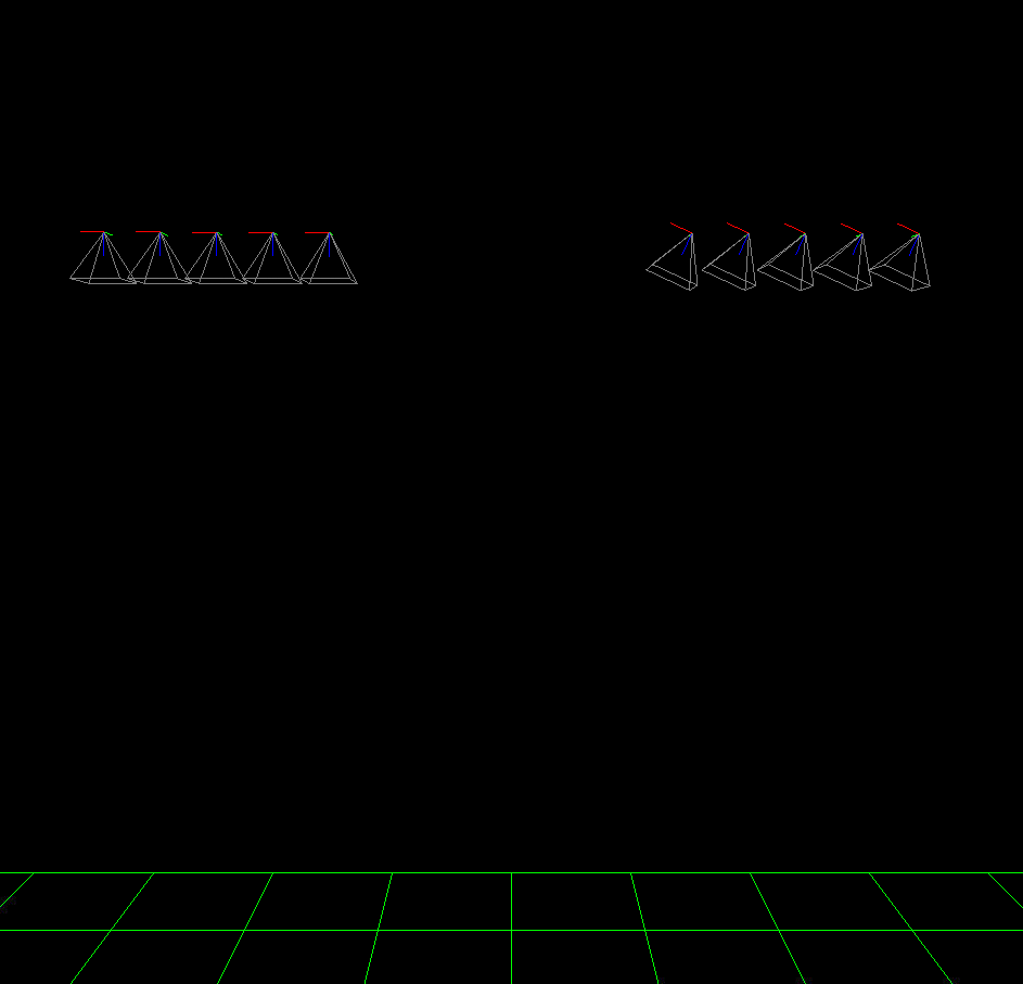
Fig. 16.26 Illustration of sat_sim creating two sets of cameras, with different fixed orientations for each, with both sets looking at the same ground path. A separate invocation of sat_sim is needed for each set.

16.60.6. Jitter modelling

As a satellite moves in orbit, it vibrates ever so slightly. The effect of this on the acquired images is called jitter, and it occurs for both Linescan and Pinhole cameras. See Section 16.37 for how jitter is solved for when the cameras are Linescan. Here we will discuss modeling jitter for synthetic Pinhole cameras. See Section 16.60.7 for how to create synthetic Linescan cameras (with or without jitter).

We assume the jitter is a superposition of periodic perturbations of the roll, pitch, and yaw angles. For each period, there will be an individual amplitude and phase shift for these three angles. For example, to model along-track (pitch) jitter only, the amplitudes for the other angles can be set to zero. Across-track jitter is modeled by a roll perturbation.

The jitter frequency will be measured in Hz. For example, f = 45 Hz (45 oscillations per second). If the satellite velocity is v meters per second, the jitter period in meters is \(v / f\). More than one jitter frequency (hence period) can be specified. Their contributions will be summed up.

Denote by \(A_{ij}\) the jitter amplitude, in degrees. The index \(i\) corresponds to jitter frequency \(f_i\), and \(j\) = 1, 2, 3 is the index for roll, pitch, and yaw. The jitter perturbation is modeled as:

\[\sum_i A_{ij} \sin\left(d \frac{2 \pi f_i}{v} + \phi_{ij}\right)\]

Some care is needed to define the parameter d. We set it to be the distance from the starting orbit point as specified by --first to the current camera center (both in ECEF, along the curved orbit). This starting point is before adjusting the orbital segment for roll, pitch, yaw, and ground constraints (Section 16.60.5).

This way the jitter amplitude at the adjusted starting point (first camera position) is uncorrelated between several sets of cameras along the same orbit but with different values of roll, pitch, yaw.

The phase shift \(\phi_{ij}\) is measured in radians. If not specified, it is set to zero. How to set it is discussed below.

16.60.6.1. Specifying the jitter amplitude in meters

The jitter amplitude is usually very small and not easy to measure or interpret. It can be set in micro radians, as done in Section 16.60.6.2.

Here we will discuss how jitter can be defined indirectly, via its effect on the horizontal uncertainty of the intersection of a ray emanating from the camera center with the datum (see also Section 14).

Consider a nadir-facing camera with the camera center at height D meters above the datum. If the ray pointing straight down from that camera intersects the datum at a certain point, and then that ray is perturbed by \(A\) degrees, the intersection point will move horizontally by

\[H = D \tan\left( \frac{\pi}{180} A \right)\]

This is the horizontal ground uncertainty of the intersection point. It is a rather intuitive concept and many vendors publish it for their cameras. For example, if the camera ground sample distance (pixel size on the ground) is 1 m/pixel, a horizontal uncertainty of 0.1 m or less is very good. If the camera orientation is found using a star-tracker or some other estimations in orbit, and no bundle adjustment (Section 16.5) is performed, the horizontal uncertainty will likely be much larger, for example on the order of 1-4 meters.

In either case, this number is easy to understand, and the jitter amplitude can be defined as the value of \(A_{ij}\) that produces the desired horizontal uncertainty:

\[A_{ij} = \frac{180}{\pi} \arctan\left( \frac{H_j}{D} \right)\]

Note that we will use the same jitter amplitude for all frequencies, since we are limited by just a single horizontal uncertainty value for each of roll, pitch, and yaw.

One should also note that the effect of a yaw perturbation by a given amount is much less than the effect of the same amount of roll or pitch perturbation, because for the latter two the effect is magnified by the distance from the camera center to the datum, unlike for yaw.

The height above datum for the starting and ending points of the orbital segment is the third value in --first and --last. These values can, in principle, be different, and then a linearly interpolated value will be used at each camera position (and note that the orbital segment endpoints are adjusted, per Section 16.60.5).

As an example of using this functionality, consider the sat_sim invocation as in Section 16.60.5, and add the options:

--velocity 7500 --jitter-frequency "45.0 100.0" \
--horizontal-uncertainty "0.0 2.0 0.0"

This will produce a set of cameras with along-track (pitch) jitter only. Two frequencies will be used, of 45 and 100 Hz.

To add a phase \(\phi_{ij}\), in radians, to roll, pitch, and yaw jitter, specify it as:

--jitter-phase "1.5708 1.5708 1.5708 0.0 0.0 0.0"

Here we used an approximation of \(\pi/2\) radians, which is 90 degrees, for the 45 Hz frequency, and 0 radians for the 100 Hz frequency.

See Section 16.60.12 for more information on these options.

A useful test is compare a camera without jitter with the corresponding one with jitter. For that, project a pixel from the first camera to the datum, and project the obtained point back into the second camera. See how different the produced pixel value is compared to the original pixel. That is done with cam_test (Section 16.9):

cam_test --session1 pinhole        \
  --session2 pinhole               \
  --image sim_jitter0/n-10020.tif  \
  --cam1  sim_jitter0/n-10020.tsai \
  --cam2  sim_jitter2/n-10020.tsai

It will produce an output as:

cam1 to cam2 pixel diff
Min:    1.89408
Median: 1.89408
Max:    1.89408

cam2 to cam1 pixel diff
Min:    1.89408
Median: 1.89408
Max:    1.89408

16.60.6.2. Specifying the jitter amplitude in micro radians

Alternatively, instead of three horizontal uncertainties, the full set of amplitudes can be specified directly, in micro radians. The option for that is --jitter-amplitude. Use a quoted list of values separated by commas of spaces. The first three values are for roll, pitch and yaw of the first frequency, the next three values are for the second frequency, and so on. For example:

--jitter-amplitude "0 1 0 0 1 0"

These will be multiplied by 1e-6 to convert to radians, then converted to degrees, and used as the jitter amplitudes \(A_{ij}\). In this example only the pitch amplitudes are nonzero, and are equal to 1 micro radian.

16.60.7. Linescan cameras

The sat_sim tool can be used to simulate Linescan cameras, with or without jitter. Then, instead of many Pinhole cameras and/or images along the orbit, a single Linescan camera and/or image will be created.

The option --num (or --frame-rate) will control how many camera samples are created between the first and last image lines (including these lines). An additional set of camera samples will be created, with the same total size, before the first and after the last image line, evenly divided between the two, to help with along-track pose interpolation and jitter modeling.

Lagrange interpolation (with 8th degree polynomials) will be used in between the samples.

All above modes are supported. One has to add to sat_sim the option --sensor-type linescan.

Add the option --square-pixels to autocompute and override the input image height (number of scan lines, the second value in --image-size) to ensure that the horizontal and vertical ground sample distances are very similar. The produced image height will be the same regardless of amount of jitter in the input cameras or whether jitter is modeled at all.

When creating synthetic linescan cameras, the row coordinate of the optical center (the second value in --optical-center) will be ignored and will be treated as set to 0. Hence, we assume that the ray from the camera center that is perpendicular to the sensor plane intersects the single-row sensor array.

The produced Linescan camera is in the CSM model state format (Section 8.12.6). This is a standard CSM format and can be read by all ASP tools including this one.

Here is an example invocation. The use case here is as in Section 16.60.5. The camera maintains fixed roll, pitch, and yaw, and the ground path determines the orbital segment endpoints. Here we also model along-track jitter.

sat_sim --dem dem.tif                \
  --ortho ortho.tif                  \
  --first 397.1 400.7 450000         \
  --last  397.1 500.7 450000         \
  --first-ground-pos 397.1 400.7     \
  --last-ground-pos  397.1 500.7     \
  --roll 0 --pitch 30 --yaw 0        \
  --num 5                            \
  --focal-length 450000              \
  --optical-center 500 500           \
  --image-size 1000 1000             \
  --sensor-type linescan             \
  --square-pixels                    \
  --jitter-frequency 5               \
  --velocity 7500                    \
  --horizontal-uncertainty '0 2 0'   \
  --jitter-phase "0.4 0.8 1.2"       \
  -o jitter2/run

Note that the image height will be overridden given the --square-pixels option.

See Section 16.37.9 for how such cameras can be used with ASP’s jitter solver.

As in Section 16.60.6.1, one can compare cameras with and without jitter as:

cam_test                   \
  --session1 csm           \
  --session2 csm           \
  --image jitter0/run.tif  \
  --cam1  jitter0/run.json \
  --cam2  jitter2/run.json

16.60.8. Roll, pitch, and yaw

The roll, pitch and yaw angles (measured in degrees) are used to determine the camera orientation relative to the local coordinate system in orbit.

When all these are set to 0 (the default is NaN) the camera looks straight down.

If the pitch is 90 degrees and the other angles are zero, the camera will look along the track rather than down. If a non-zero yaw is set, the camera will rotate around its view axis.

The rotations are applied to the camera body in the roll, pitch, and yaw order. So, the combined rotation matrix is:

R = yawRot * pitchRot * rollRot

(the application is from right to left). The camera-to-ECEF rotation is produced by further multiplying this matrix on the left by the rotation from the local satellite coordinate system to ECEF.

It is important to note that the satellite and the camera use different coordinate systems. The satellite orientation is with the x, y and z axes pointing along satellite track, across track, and towards the planet, respectively.

For the camera, it is preferable for the rows of pixels to be parallel to the across track direction, and for the columns to be parallel to the along track direction. So, the camera y direction is along the track, the camera x direction is the negative of the across-track direction, and z points towards the ground as before.

16.60.9. Efficiency considerations

Each image (of size about 2000 x 1000 pixels) can take about 10 seconds to create using multiple threads. A job can be divided over several processes using the --first-index and --last-index options (see Section 16.60.12). The last index is the index before the last camera. The option --no-images can be used to skip the image creation step.

16.60.10. Preparing the input DEM and orthoimage

The input DEM must not have holes, be reasonably smooth, and extend well-beyond the area of interest. It is suggested to create it using stereo (Section 3). For steep terrain one should first mapproject the images (Section 6.1.7).

The stereo cloud should be converted to a DEM, preferably in the local stereographic projection, using a grid size that is perhaps 4 times the ground sample distance (GSD). For example, for images having a GSD of 0.4 meters, a command as follows may work (adjust the actual projection center and datum to your location):

proj='+proj=stere +lat_0=-25.34361 +lon_0=131.0329 +k=1 +x_0=0 +y_0=0 +datum=WGS84 +units=m +no_defs'
point2dem --t_srs "$proj" --tr 1.6 run/run-PC.tif

The dem_mosaic (Section 16.19) tool can be used to fill holes in the DEM, using either the --hole-fill-length or --fill-search-radius option. It is also suggested to blur it a little, which may reduce some of the noise in the DEM. For that, use dem_mosaic with the option --blur-sigma with a value of 1 or 2.

Very large holes may be infilled from a third-party low-resolution DEM, like Copernicus (Section 6.1.7.1), but this is a measure of last resort. Do not forget to first convert it to be relative to the WGS84 ellipsoid, using dem_geoid (Section 6.1.7.2). This DEM can be converted to the local projection and grid size using gdalwarp (Section 16.24, bicubic or bilinear interpolation is suggested), and cropped to desired area with gdal_translate. Then, it can be used as:

dem_mosaic --priority-blending-length 100 \
  stereo-DEM.tif copernicus-DEM.tif       \
  -o filled-DEM.tif

This assumes that the two DEMs being blended are reasonably well-aligned. Otherwise, alignment may be needed (Section 16.52).

One can also use such a third party DEM if no stereo DEM can be produced.

The orthoimage can be obtained by mapprojecting (Section 16.40) a satellite image onto the DEM at the native resolution of the image:

mapproject --t_srs "$proj" --tr 0.4 -t rpc filled-DEM.tif \
  image.tif image.xml ortho.tif

Here we assumed a WorldView satellite, so option -t rpc was used. See Section 6.1.7.8 for how to handle other satellites.

16.60.11. Output files

In addition to the images and/or cameras, when --sensor-type is pinhole, sat_sim will also save two files, having the lists of created images and cameras, one per line, with names as:

<output prefix>-images.txt
<output prefix>-cameras.txt

These files will not be saved if --first-index is non-zero, as then sat_sim is presumably being invoked concurrently by several processes to write several ranges of images and/or cameras, and that may result in these files being corrupted.

Then, the list of images will not be saved if --no-images is used, and the list of cameras will not be saved if --camera-list is set, as then the cameras are not being generated by sat_sim.

16.60.12. Command-line options

--dem <string (default=””)>

Input DEM file.

--ortho <string (default=””)>

Input georeferenced image file.

-o, --output-prefix <string (default=””)>

Specify the output prefix. All the files that are saved will start with this prefix.

--camera-list <string (default=””)>

A file containing the list of pinhole cameras to create synthetic images for. Then these cameras will be used instead of generating them. Specify one file per line. The options --first, --last, --num, --focal-length, and --optical-center will be ignored.

--first <float, float, float>

First camera position, specified as DEM pixel column and row, and height above the DEM datum. This may be adjusted, per Section 16.60.5.

--last <float, float, float>

Last camera position, specified as DEM pixel column and row, and height above the DEM datum. See also --first.

--num <int (default=0)>

Number of cameras to generate, including the first and last ones. Must be positive. The cameras are uniformly distributed along the straight edge from first to last (in projected coordinates). See also --frame-rate.

--first-ground-pos <float, float>

Coordinates of first camera ground footprint center (DEM column and row). If not set, the cameras will look straight down (perpendicular to along and across track directions).

--last-ground-pos <float, float>

Coordinates of last camera ground footprint center (DEM column and row). If not set, the cameras will look straight down (perpendicular to along and across track directions).

--focal-length <double>

Output camera focal length in units of pixel.

--optical-center <float, float>

Output camera optical center (image column and row). Units of pixel.

--image-size <int, int>

Output camera image size (width and height).

--roll <double>

Camera roll angle, in degrees. See Section 16.60.4 for details.

--pitch <double>

Camera pitch angle, in degrees. See Section 16.60.4 for details.

--yaw <double>

Camera yaw angle, in degrees. See Section 16.60.4 for details.

--velocity <double>

Satellite velocity, in meters per second. Used for modeling jitter. A value of around 8000 m/s is typical for a satellite like SkySat in Sun-synchronous orbit (90 minute period) at an altitude of about 450 km. For WorldView, the velocity is around 7500 m/s, with a higher altitude and longer period.

--jitter-frequency <string>

Jitter frequency, in Hz. Used for modeling jitter (satellite vibration). Several frequencies can be specified. Use a quoted list, with spaces or commas as separators. See also --jitter-amplitude and --horizontal-uncertainty.

--jitter-phase <string>

Jitter phase, in radians. Measures the jitter phase offset from the start of the orbit as set by --first. Specify as a quoted list of numbers. Number of values must be 3 times the number of frequencies. The order in this list corresponds to phase for roll, pitch, and yaw for first frequency, then second frequency, etc. If not specified, will be set to 0.

--jitter-amplitude <string>

Jitter amplitude, in micro radians. Specify as a quoted list having amplitude in roll, pitch, yaw for first frequency, then second frequency, etc. Separate the values by spaces or commas.

--horizontal-uncertainty <string>

Camera horizontal uncertainty on the ground, in meters, at nadir orientation. Specify as three numbers, in quotes, used for roll, pitch, and yaw. The jitter amplitude for each of these angles is found as amplitude = atan(horizontal_uncertainty / satellite_elevation_above_datum), then converted to degrees. See Section 16.60.6 for details.

--frame-rate <double>

Camera frame rate, per second. Can be in double precision. If set, it will override --num. The cameras will start from --first (after any position adjustment, if applicable, per Section 16.60.5). Set the --velocity value. The last camera will be no further than the (adjusted) value of --last along the orbit.

--sensor-type <string (default=”pinhole”)>

Sensor type for created cameras and images. Can be one of: pinhole, linescan.

--square-pixels

When creating linescan images, override the image height (the second value in --image-size) to ensure that the horizontal and vertical ground sample distances are very similar.

--first-index <int (default: -1)>

Index of first camera and/or image to generate, starting from 0. If not set, will create all images/cameras. This is used for parallelization.

--last-index <int (default: -1)>

Index of last image and/or camera to generate, starting from 0. Stop before this index. If not set, will create all images/cameras. This is used for parallelization.

--no-images

Create only cameras, and no images. Cannot be used with --camera-list.

--save-ref-cams

For each created camera, save also the ‘reference’ camera that has no roll, pitch, yaw, jitter, or 90 degree in-sensor-plane rotation from camera to satellite coordinates. Their names have -ref- after the output prefix.

--save-as-csm

Save Pinhole (frame) cameras in the CSM format, as done for linescan cameras. Can be used to combine these sensors in bundle adjustment and solving for jitter. See an example in Section 16.37.11.

--dem-height-error-tol <float (default: 0.001)>

When intersecting a ray with a DEM, use this as the height error tolerance (measured in meters). It is expected that the default will be always good enough.

--threads <integer (default: 0)>

Select the number of threads to use for each process. If 0, use the value in ~/.vwrc.

--cache-size-mb <integer (default = 1024)>

Set the system cache size, in MB.

--tile-size <integer (default: 256 256)>

Image tile size used for multi-threaded processing.

--tif-compress <string (default = “LZW”)>

TIFF compression method. Options: None, LZW, Deflate, Packbits.

-v, --version

Display the version of software.

-h, --help

Display this help message.