11.1. Overview of SfS
ASP provides a tool, named sfs (Section 16.67), that can improve the level
of detail of DEMs created by ASP or any other source using shape-from-shading
(SfS). This program takes as input one or more images and cameras, a DEM at
roughly the same resolution as the images, and returns a refined DEM.
The modeling approach is described in [AB18].
The sfs program works with any cameras supported by ASP, for Earth and other
planets. The option --sun-angles can be used to specify the Sun
information for each image. For ISIS and CSM cameras, if this option is not set,
the needed information is read from the camera files.
The sfs program can model position-dependent albedo (Section 11.8),
exposure values for each camera, atmospheric haze, shadows in the input images,
and regions in the DEM occluded from the Sun.
A program named parallel_sfs is provided (Section 16.50)
that parallelizes sfs using multiple processes (optionally on
multiple machines) by splitting the input DEM into tiles with padding,
running sfs on each tile, and then blending the results. It was used
to create DEMs of dimensions 10,000 by 10,000 pixels.
11.2. Examples
A single image example with LRO NAC Lunar images (Section 11.7).
A small example with multiple LRO NAC images (Section 11.9).
Large-scale SfS with LRO NAC images (Section 11.10).
Kaguya Lunar images (Section 8.14.5).
Earth example, with atmospheric haze (Section 11.12).
CTX Mars example (Section 11.13).
11.3. Limitations
This program is experimental. It assumes a certain reflectance model of the surface, which may or may not be accurate for a given setting.
sfs is very sensitive to errors in the position and
orientation of the cameras, the accuracy of the initial DEM, and to
the value of the weights it uses.
sfs has been tested thoroughly with Lunar LRO NAC datasets.
As can be seen below, sfs returns reasonable results on the Moon
as far as 85 degrees and even 89.6 degrees South.
SfS was shown to give reasonable results with CTX Mars images (Section 11.13). The improvement is real, but somewhat modest.
An example for Earth is Section 11.12, that shows that our program can give plausible results.
It is suggested to invoke this tool with a terrain model that is
already reasonably accurate, and with images with diverse illumination
conditions registered to it, when sfs can do fine-level
refinements.
The program was employed successfully for Mercury ([BMB+23]). Applications for the Moon are described in [HIK+25] and [Boa24].
11.4. Mathematical model
This program works by minimizing the cost function
Here, \(I_k(\phi(x, y))\) is the \(k\)-th camera image interpolated at pixels obtained by projecting into the camera 3D points from the terrain \(\phi(x, y)\), \(T_k\) is the \(k\)-th image exposure, \(A(x, y)\) is the per-pixel normalized albedo, \(R_k(\phi(x, y))\) is the reflectance computed from the terrain for \(k\)-th image, \(\left\|\nabla^2 \phi(x, y) \right\|^2\) is the sum of squares of all second-order partial derivatives of \(\phi\).
The term \(H_k\) is the atmospheric haze, which is assumed to be zero for the Moon but is modeled for Earth and Mars.
The value \(\mu > 0\) is a smoothness weight, and \(\lambda > 0\) determines how close we should stay to the input terrain \(\phi_0\) (smaller \(\mu\) will show more detail but may introduce some artifacts, and smaller \(\lambda\) may allow for more flexibility in optimization but the terrain may move too far from the input).
We use either the regular Lambertian reflectance model, or the Lunar-Lambertian model [McE91], more specifically as given in [LHK06] (equations (3) and (4)). Also supported is the Hapke model, [JGL+06], [FSC+13], [Hap08], [HNS93]. Custom values for the coefficients of these models can be passed to the program.
Note that the albedo in the above expression is normalized, its nominal value is 1. The image intensity ideally equals the image exposure times albedo times reflectance, hence the image exposure absorbs any existing constant multiplier.
The exposure value for a camera is computed as the average of the image
intensity divided by the average reflectance, both computed over the DEM.
If the problem is parallelized using parallel_sfs, the exposures
are found just once, over the entire DEM, rather than for each tile.
The exposures can be optimized while solving for the DEM.
It is important to note that the default Lunar-Lambertian model may not be the right choice for other planetary bodies, hence some research may be needed to decide the correct model for your application.
11.5. How to get images
We obtain the images from http://wms.lroc.asu.edu/lroc/search (search for EDR images of type NACL and NACR).
A faster (but not as complete) interface is provided by http://ode.rsl.wustl.edu/moon/indexproductsearch.aspx. This site allows for bulk downloads, but does not permit datasets bigger than several tens of GB, so several attempts may be necessary.
The related site http://ode.rsl.wustl.edu/moon/indextools.aspx?displaypage=lolardr can provide LOLA datasets which can be used as (sparse) ground truth.
If desired to use a gridded LOLA DEM as an initial guess, see Section 11.10.
We advise the following strategy for picking images. First choose a
small longitude-latitude window in which to perform a search for
images. Pick two images that are very close in time and with a big
amount of overlap (ideally they would have consecutive orbit numbers).
A good convergence angle is expected (Section 8.1).
Those images can be passed to ASP’s parallel_stereo tool to create an
initial DEM. Then, search for other images close to the center of the
maximum overlap of the first two images. Pick one or more of those,
ideally with different illumination conditions than the first
two. Those (together with one of the first two images) can be used for
SfS.
To locate the area of spatial overlap, the images can be map-projected
(either with cam2map at a coarse resolution, or with
mapproject), using for example the LOLA DEM as the terrain to
project onto, or the DEM obtained from running parallel_stereo on
those images. Then the images can be overlaid as georeferenced images
in stereo_gui (Section 16.72). A good sanity check is to
examine the shadows in various images. If they point in different
directions in the images and perhaps also have different lengths, that
means that illumination conditions are different enough, which will
help constrain the sfs problem better.
An example for how to download and prepare the datasets is shown in Section 11.7.
11.6. ISIS vs CSM models
CSM (Section 8.12) is a modern sensor model which can be used with
multiple threads, and can be on the order of 7-15 times faster than the
ISIS .cub model it is meant to replace, as benchmarked with
mapproject, bundle_adjust, and sfs.
Given a set of ISIS .cub camera files it is desired to run SfS on, it is strongly suggested to convert them to corresponding CSM models as described in Section 8.12.2.1.
If the CSM models have no more than 0.5 pixels of discrepancy when compared to
the .cub cameras, as validated with cam_test (Section 16.9), use the
CSM models instead of the ISIS ones in all the tools outlined below
(parallel_bundle_adjust, parallel_stereo, mapproject, and
parallel_sfs). The SfS DEMs obtained with these two methods were observed to
differ by several millimeters at most, on average, but an evaluation may be
necessary for your particular case.
This will work only for the datasets with original dimensions, so
not together with the reduce or crop commands.
Any of the commands further down which only use .cub files can be adapted for use with CSM cameras by appending to those commands the CSM .json cameras in the same order as the .cub files, from which only the image information will then be used, with the camera information coming from the .json files.
For example, if sfs is run with an ISIS camera as:
sfs --use-approx-camera-models\
 --crop-input-images          \
  -i input_dem.tif image.cub  \
  -o sfs_isis/run
then, the corresponding command using the CSM model will be:
sfs --crop-input-images \
  -i input_dem.tif      \
  image.cub image.json  \
  -o sfs_csm/run
The option --use-approx-camera-models is no longer necessary
as the CSM model is fast enough. It is however suggested to still
keep the --crop-input-images option.
Bundle adjustment saves CSM camera files with adjustments already applied to
them, so the resulting cameras can be used without the
--bundle-adjust-prefix option.
11.7. SfS at 1 meter/pixel using a single image
In both this and the next sections we will work with LRO NAC images taken close to the Lunar South Pole, at a latitude of 85 degrees South (the tool was tested on equatorial regions as well). We will use four images, M139939938LE, M139946735RE, M173004270LE, and M122270273LE.
11.7.1. Data preparation
Fetch the images:
wget http://lroc.sese.asu.edu/data/LRO-L-LROC-2-EDR-V1.0/LROLRC_0005/DATA/SCI/2010267/NAC/M139939938LE.IMG
wget http://lroc.sese.asu.edu/data/LRO-L-LROC-2-EDR-V1.0/LROLRC_0005/DATA/SCI/2010267/NAC/M139946735RE.IMG
wget http://lroc.sese.asu.edu/data/LRO-L-LROC-2-EDR-V1.0/LROLRC_0009/DATA/SCI/2011284/NAC/M173004270LE.IMG
wget http://lroc.sese.asu.edu/data/LRO-L-LROC-2-EDR-V1.0/LROLRC_0002/DATA/MAP/2010062/NAC/M122270273LE.IMG
We convert these to ISIS cubes, initialize the SPICE kernels, and perform radiometric calibration and echo correction. That is explained in Section 8.7.4.
It can be convenient to create preview versions of these datasets, at 10% of original resolution, for the purpose of inspection. That is done as follows:
f=M139939938LE
reduce from = ${f}.cal.echo.cub to = ${f}.cal.echo.sub10.cub  \
  sscale = 10 lscale = 10
For simplicity, we create shorter aliases for these images:
ln -s M139939938LE.cal.echo.cub A.cub
ln -s M139946735RE.cal.echo.cub B.cub
ln -s M173004270LE.cal.echo.cub C.cub
ln -s M122270273LE.cal.echo.cub D.cub
11.7.2. Initial DEM creation
The first step is to run bundle adjustment (Section 16.5) and stereo (Section 16.51) to create an initial guess DEM. We picked for this the first two of these images. These form a stereo pair (Section 8.1), that is, they have a reasonable baseline and sufficiently close times of acquisition hence very similar illuminations. These conditions are necessary to obtain a good stereo result.
Below we assume CSM cameras are used (Section 11.6).
Otherwise the .json files should be omitted.
bundle_adjust A.cub B.cub A.json B.json   \
  --num-iterations 100 -o ba/run

parallel_stereo                           \
  --left-image-crop-win 0 7998 2728 2696  \
  --right-image-crop-win 0 9377 2733 2505 \
  --stereo-algorithm asp_mgm              \
  --subpixel-mode 9                       \
  --bundle-adjust-prefix ba/run           \
  A.cub B.cub A.json B.json               \
  run_full1/run
See Section 6.1 for a discussion about various speed-vs-quality choices in stereo. See Section 6.1.7 about handling artifacts in steep terrain.
The crop windows above were chosen with stereo_gui (Section 16.72).
Next we create a DEM. We use the stereographic projection since this dataset is very close to the South Pole. Normally a projection centered close to area of interest is suggested (Section 16.56.1).
point2dem -r moon --stereographic --proj-lon 0  \
  --proj-lat -90 run_full1/run-PC.tif
It is very important that the resolution of the DEM be comparable to the ground sample distance (GSD) of the images. This will ensure optimal sampling.
SfS can only be run on a DEM with valid data at each grid point. The
DEM obtained above should be opened in stereo_gui, and the bounds
of a clip having only valid data should be determined
(Section 16.72.8). Such a clip is cropped using
gdal_translate (Section 16.25) as:
gdal_translate -projwin -15471.9 150986 -14986.7 150549  \
  run_full1/run-DEM.tif run_full1/run-crop-DEM.tif
This creates a DEM clip of size 456 × 410 pixels.
The point2dem program auto-determines the DEM resolution (grid
size), as an estimate of the image ground sample distance
(GSD). This is the optimal resolution to run SfS at. If creating your
input DEM some other way, it is strongly suggested to use a DEM grid
size not too different from the GSD, in order to get the best
quality. The mapproject program (Section 16.41), when
invoked with no input grid size, computes the grid size as the image
GSD, and that value can then be used when creating the input SfS DEM.
If this DEM has holes, those can be filled in dem_mosaic
(Section 16.20.2.9).
The dem_mosaic program can also apply some blur to attenuate big artifacts
(Section 16.20.2.6). Use, for example, --dem-blur-sigma 2. Note that
sfs has a smoothness term which should take care of very small
imperfections in the input.
See Section 11.10.2 for how to use a third-party DEM as input to SfS. Then, alignment of the cameras to that DEM is needed. This is a multi-step process, outlined in detail in Section 11.10.
11.7.3. Running SfS
Then we run sfs on this clip (for a larger clip parallel_sfs
should be used instead, see Section 16.50):
sfs -i run_full1/run-crop-DEM.tif       \
  A.cub A.json                          \
  --use-approx-camera-models            \
  --crop-input-images                   \
  --reflectance-type 1                  \
  --smoothness-weight 0.08              \
  --initial-dem-constraint-weight 0.001 \
  --max-iterations 10                   \
  -o sfs_ref1/run
The smoothness weight is a parameter that needs tuning. If it is too small, SfS will return noisy results, if it is too large, too much detail will be blurred. One can experiment with values between 0.01 and 100,000 with a factor of 10 to find this weight, and then refine it in smaller steps. A discussion of this term is in [LSAM21].
Here we used the Lunar-Lambertian model. The meaning of the other sfs
options can be looked up in Section 16.67.
Normally 5-10 iterations is enough, even when convergence is not reached, as the solution usually improves quickly at first and only very fine refinements happen later.
The value of --initial-dem-constraint-weight is best set to something very
small when the initial DEM is not very reliable, as otherwise defects from it
can be inherited by the SfS result. Otherwise a value between 0.001 and 0.002
may be good enough. Use a higher value when the input DEM is reliable but the
reflectance model is not.
See Section 11.8 for modeling of albedo. Shadow thresholds may be needed to avoid artifacts in shadow. See Section 11.9.2 for a potential solution to flat crater bottoms in areas in shadow.
In the next sections, where SfS will be done with multiple images, more parameters which can control the quality of the result will be explored.
See Section 16.67.5 for where sfs stores its outputs.
See Section 8.14.5 for an example of running SfS on Kaguya TC images.
11.7.4. Inspecting the results
We show the results of running this program in Fig. 11.1. The
left-most figure is the hill-shaded original DEM, which was obtained
by running the hillshade program (Section 16.28):
hillshade --azimuth 300 --elevation 20 run_full1/run-crop-DEM.tif \
  -o run_full1/run-crop-hill.tif
The second image is the hill-shaded DEM obtained after running sfs
for 10 iterations.
The third image is, for comparison, the map-projection of A.cub onto the original DEM, obtained via the command:
mapproject --tr 1 run_full1/run-crop-DEM.tif A.cub A_map.tif \
  --tile-size 1024
(For small DEMs one can use a smaller --tile-size to start more
subprocesses in parallel to do the mapprojection. That is not needed
with CSM cameras as then mapproject is multithreaded.)
The fourth image is the colored absolute difference between the
original DEM and the SfS output, obtained by running geodiff
(Section 16.26):
geodiff --absolute sfs_ref1/run-DEM-final.tif \
  run_full1/run-crop-DEM.tif -o out
colormap --min 0 --max 2 out-diff.tif
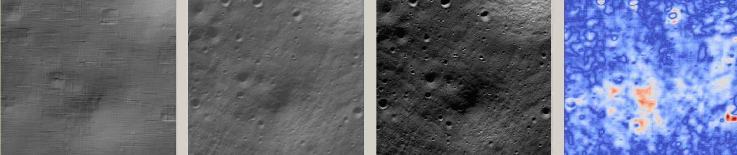
Fig. 11.1 An illustration of sfs. The images are, from left to right, the
original hill-shaded DEM, the hill-shaded DEM obtained from sfs,
the image A.cub map-projected onto the original DEM, and the absolute
difference of the original and final DEM, where the brightest shade
of red corresponds to a 2 meter height difference.
It can be seen that the optimized DEM provides a wealth of detail and looks quite similar to the input image. It also did not diverge significantly from the input DEM. We will see in the next section that SfS is in fact able to make the refined DEM more accurate than the initial guess (as compared to some known ground truth), though that is not guaranteed, and most likely did not happen here where just one image was used.
11.8. Albedo modeling with one or more images
When using a single input image, it may be preferable to avoid floating
(solving for) the albedo (option --float-albedo), hence to have it
set to 1 and kept fixed. The reason for that is because for a single
image it is not possible to distinguish if a bright image area comes
from lighter-colored terrain or from having an inclination which makes
it face the Sun more.
If desired to float the albedo with one image, it is suggested to use
a higher value of --initial-dem-constraint-weight to constrain the
terrain better in order to make albedo determination more reliable.
The albedo can be prevented from changing too much if the
--albedo-constraint-weight parameter is used.
Albedo should be floated with two or more images, if albedo variations are clearly visible, and if those images have sufficiently different illumination conditions, as then the albedo and slope effects can be separated more easily. For images not having obvious albedo variations it may be prudent to keep the albedo fixed at the nominal value of 1.
It is important to use appropriate values for the
--shadow-thresholds parameter, as otherwise regions in shadow will
be interpreted as lit terrain with a pitch-black color, and the computed
albedo and terrain will have artifacts.
See Section 16.67.5 for the produced file having the albedo.
An example showing modeling of albedo (and atmospheric haze) is in Section 11.12.
11.9. SfS with multiple images in the presence of shadows
In this section we will run sfs with multiple images. We would
like to be able to see if SfS improves the accuracy of the DEM rather
than just adding detail to it. We evaluate this using the following
(admittedly imperfect) approach. We reduce the resolution of the
original images by a factor of 10, run stereo with them, followed by
SfS using the stereo result as an initial guess and with the resampled
images. As ground truth, we create a DEM from the original images at
the higher resolution of 1 meter/pixel, which we bring closer to the
initial guess for SfS using pc_align. We would like to know if
running SfS brings us even closer to this “ground truth” DEM.
The most significant challenge in running SfS with multiple images is that shape-from-shading is highly sensitive to errors in camera position and orientation. It is suggested to bundle-adjust the cameras first (Section 16.5).
It is important to note that bundle adjustment may fail if the images have very different illumination, as it will not be able to find matches among images. A solution to this is discussed in Section 11.10, and it amounts to bridging the gap with more images of intermediate illumination.
It is strongly suggested that, when doing bundle adjustment, the images should be specified in the order given by Sun azimuth angle (see Section 11.10.5). The images should also be mapprojected and visualized (in the same order), to verify that the illumination is changing gradually.
To make bundle adjustment and stereo faster, we first crop the images,
such as shown below (the crop parameters can be determined via
stereo_gui, Section 16.72).
crop from = A.cub to = A_crop.cub sample = 1 line = 6644 \
  nsamples = 2192 nlines = 4982
crop from = B.cub to = B_crop.cub sample = 1 line = 7013 \
    nsamples = 2531 nlines = 7337
crop from = C.cub to = C_crop.cub sample = 1 line = 1    \
  nsamples = 2531 nlines = 8305
crop from = D.cub to = D_crop.cub sample = 1 line = 1    \
  nsamples = 2531 nlines = 2740
Note that manual cropping is not practical for a very large number of
images. In that case, it is suggested to mapproject the input images
onto some smooth DEM whose extent corresponds to the terrain to be
created with sfs (with some extra padding), then run bundle
adjustment with mapprojected images (option --mapprojected-data,
illustrated in Section 11.10) and stereo also with
mapprojected images (Section 6.1.7). This will not only be
automated and faster, but also more accurate, as the inputs will be
more similar after mapprojection.
Bundle adjustment (Section 16.5) and stereo happens as follows:
bundle_adjust A_crop.cub B_crop.cub C_crop.cub D_crop.cub \
  --num-iterations 100 --save-intermediate-cameras        \
  --ip-per-image 20000 --max-pairwise-matches 2000        \
  --min-matches 1 --num-passes 1 -o run_ba/run
parallel_stereo A_crop.cub B_crop.cub run_full2/run       \
  --subpixel-mode 3 --bundle-adjust-prefix run_ba/run
One can try using the stereo option --nodata-value
(Section 17) to mask away shadowed regions, which may
result in more holes but less noise in the terrain created from
stereo.
See Section 6.1 for a discussion about various speed-vs-quality choices, and Section 6.1.7 about handling artifacts in steep terrain. Consider using CSM cameras instead of ISIS cameras (Section 11.6).
The resulting cloud, run_full2/run-PC.tif, will be used to create
the “ground truth” DEM. As mentioned before, we’ll in fact run SfS
with images subsampled by a factor of 10. Subsampling is done by
running the ISIS reduce command:
for f in A B C D; do
  reduce from = ${f}_crop.cub to = ${f}_crop_sub10.cub \
    sscale = 10 lscale = 10
done
We run bundle adjustment and parallel_stereo with the subsampled
images using commands analogous to the above. It was quite challenging
to find match points, hence the --mapprojected-data option in
bundle_adjust was used, to find interest matches among
mapprojected images. The process went as follows:
# Prepare mapprojected images (see note in the text below)
parallel_stereo A_crop_sub10.cub B_crop_sub10.cub \
  --subpixel-mode 3 run_sub10_noba/run
point2dem -r moon --tr 10 --stereographic         \
  --proj-lon 0 --proj-lat -90                     \
  run_sub10_noba/run-PC.tif
for f in A B C D; do
  mapproject run_sub10_noba/run-DEM.tif --tr 10   \
    ${f}_crop_sub10.cub ${f}_sub10.map.noba.tif
done

# Run bundle adjustment
bundle_adjust A_crop_sub10.cub B_crop_sub10.cub     \
  C_crop_sub10.cub D_crop_sub10.cub --min-matches 1 \
  --num-iterations 100 --save-intermediate-cameras  \
  -o run_ba_sub10/run --ip-per-image 20000          \
  --max-pairwise-matches 2000 --overlap-limit 200   \
  --match-first-to-last --num-passes 1              \
  --mapprojected-data                               \
  "$(ls [A-D]_sub10.map.noba.tif) run_sub10_noba/run-DEM.tif"
It is suggested to use above a DEM not much bigger than the eventual area of interest, otherwise interest points which are far away may be created. While that may provide robustness, in some occasions, given that LRO NAC images are very long and can have jitter, interest points far away could actually degrade the quality of eventual registration in the desired smaller area.
The same resolution should be used for both mapprojected images
(option --tr), and it should be similar to the ground sample
distance of these images.
The option --mapprojected-data assumes that the images have
been mapprojected without bundle adjustment.
The option --max-pairwise-matches in bundle_adjust should
reduce the number of matches to the set value, if too many were
created originally.
The option --overlap-limit reduces the number of subsequent images to be
matched to the current one to this value. For a large number of images consider
using the option --auto-overlap-params which will find which images overlap.
Run stereo and create a DEM:
parallel_stereo A_crop_sub10.cub B_crop_sub10.cub   \
  run_sub10/run --subpixel-mode 3                   \
 --bundle-adjust-prefix run_ba_sub10/run
 point2dem -r moon --tr 10 --stereographic          \
    --proj-lon 0 --proj-lat -90 run_sub10/run-PC.tif
This will create a point cloud named run_sub10/run-PC.tif and
a DEM run_sub10/run-DEM.tif.
It is strongly suggested to mapproject the bundle-adjusted images onto this DEM and verify that the obtained images agree:
for f in A B C D; do
   mapproject run_sub10/run-DEM.tif               \
     ${f}_crop_sub10.cub ${f}_sub10.map.yesba.tif \
     --bundle-adjust-prefix run_ba_sub10/run
 done
 stereo_gui --use-georef --single-window *yesba.tif
We’ll bring the “ground truth” point cloud closer to the initial
guess for SfS using pc_align:
pc_align --max-displacement 200 run_full2/run-PC.tif \
  run_sub10/run-PC.tif -o run_full2/run              \
  --save-inv-transformed-reference-points
This step is extremely important. Since we ran two bundle adjustment steps, and both were without ground control points, the resulting clouds may differ by a large translation, which we correct here. Hence we would like to make the “ground truth” terrain aligned with the datasets on which we will perform SfS.
Next we create the “ground truth” DEM from the aligned high-resolution point cloud, and crop it to a desired region:
point2dem -r moon --tr 10 --stereographic  \
  --proj-lon 0 --proj-lat -90              \
  run_full2/run-trans_reference.tif
gdal_translate                             \
  -projwin -15540.7 151403 -14554.5 150473 \
  run_full2/run-trans_reference-DEM.tif    \
  run_full2/run-crop-DEM.tif
We repeat the same steps for the initial guess for SfS:
point2dem -r moon --tr 10 --stereographic  \
  --proj-lon 0 --proj-lat -90              \
  run_sub10/run-PC.tif
gdal_translate                             \
  -projwin -15540.7 151403 -14554.5 150473 \
  run_sub10/run-DEM.tif                    \
  run_sub10/run-crop-DEM.tif
Since our dataset has many shadows, we found that specifying the
shadow thresholds for the tool improves the results. The thresholds
can be determined using stereo_gui. This can be done by turning on
threshold mode from the GUI menu, and then clicking on a few points in
the shadows. The largest of the determined pixel values will be the
used as the shadow threshold. Then, the thresholded images can be
visualized/updated from the menu as well, and this process can be
iterated. See Section 16.72.13 for more details. We also found that
for LRO NAC a shadow threshold value of 0.003 works well enough
usually.
Alternatively, the otsu_threshold tool (Section 16.47)
can be used to find the shadow thresholds automatically. It can
overestimate them somewhat.
Then, we run sfs:
sfs -i run_sub10/run-crop-DEM.tif                    \
  A_crop_sub10.cub C_crop_sub10.cub D_crop_sub10.cub \
  -o sfs_sub10_ref1/run --threads 4                  \
  --smoothness-weight 0.12                           \
  --initial-dem-constraint-weight 0.001              \
  --reflectance-type 1 --use-approx-camera-models    \
  --max-iterations 5  --crop-input-images            \
  --bundle-adjust-prefix run_ba_sub10/run            \
  --blending-dist 10 --allow-borderline-data         \
  --min-blend-size 20                                \
  --shadow-thresholds '0.00162484 0.0012166 0.000781663'
Varying the exposures and haze is not suggested in a first attempt.
Note the two “blending” parameters, those help where there are seams
or light-shadow boundaries. The precise numbers may need
adjustment. In particular, decreasing --min-blend-size may result
in more seamless terrain models at the expense of some erosion.
One should experiment with floating the albedo (option
--float-albedo) if noticeable albedo variations are seen in the
images. See Section 11.8 for a longer discussion.
After this command finishes, we compare the initial guess to sfs to
the “ground truth” DEM obtained earlier and the same for the final
refined DEM using geodiff as in the previous section. Before SfS:
geodiff --absolute run_full2/run-crop-DEM.tif \
  run_sub10/run-crop-DEM.tif -o out
gdalinfo -stats out-diff.tif | grep Mean=
and after SfS:
geodiff --absolute run_full2/run-crop-DEM.tif \
  sfs_sub10_ref1/run-DEM-final.tif -o out
gdalinfo -stats out-diff.tif | grep Mean=
The mean error goes from 2.64 m to 1.29 m, while the standard deviation decreases from 2.50 m to 1.29 m.
See Fig. 11.3 for an illustration. Visually the refined DEM looks more detailed. The same experiment can be repeated with the Lambertian reflectance model (reflectance-type 0), and then it is seen that it performs a little worse.
We also show in this figure the first of the images used for SfS,
A_crop_sub10.cub, map-projected upon the optimized DEM. Note that we
use the previously computed bundle-adjusted cameras when map-projecting,
otherwise the image will show as shifted from its true location:
mapproject sfs_sub10_ref1/run-DEM-final.tif A_crop_sub10.cub   \
  A_crop_sub10_map.tif --bundle-adjust-prefix run_ba_sub10/run
See Section 11.10 for a large-scale example.
11.9.1. Handling borderline areas
With the option --allow-borderline-data, sfs is able to do a
better job at resolving the terrain at the border of regions that have
no lit pixels in any images. It works by not letting the image
blending weights decay to 0 at this boundary, which is normally the
case when --blending-dist is used. These weights still decrease
to 0 at other image boundaries.
In the example in Fig. 11.2, in some input images the top terrain portion was lit, and in some the bottom portion. With this option, as it can be seen, the blur in the transition zone is removed. The craters are still too shallow, but that is a known issue with weak illumination, and something to be addressed at a future time.
The value of --blending-dist should be set to 10 or so. A smaller
value may result in seams. Increasing this will allow the seams to be
attenuated, but may result in more erosion.
The sfs_blend tool (Section 16.68) can be used to tune
the areas in complete shadow after doing SfS.
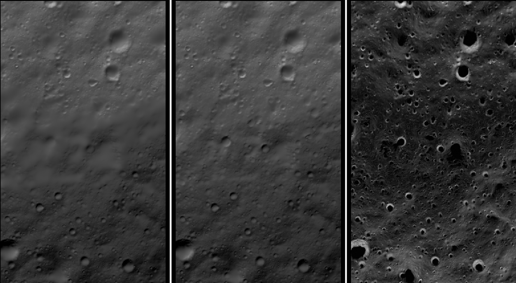
Fig. 11.2 The SfS result without option --allow-borderline-data (left),
with it (center), and the max-lit mosaic (right). It can be seen
in the max-lit mosaic that the illumination direction (position of
lit crater rim) is quite different in the top and bottom halves
(which appear to be separated by a horizontal ridge), which was
causing issues for the algorithm.
11.9.2. Handling lack of data in shadowed crater bottoms
As seen in Fig. 11.3, sfs makes the crater bottoms
flat in shadowed areas, where is no data.
A very experimental way of fixing this is to add a new curvature term in the areas in shadow, of the form
to the SfS formulation in Section 11.4. As an example, running:
sfs -i run_sub10/run-crop-DEM.tif                      \
    A_crop_sub10.cub C_crop_sub10.cub D_crop_sub10.cub \
    -o sfs_sub10_v2/run                                \
    --threads 4 --smoothness-weight 0.12               \
    --max-iterations 5                                 \
    --initial-dem-constraint-weight 0.001              \
    --reflectance-type 1                               \
    --use-approx-camera-models                         \
    --crop-input-images                                \
    --bundle-adjust-prefix run_ba_sub10/run            \
    --shadow-thresholds '0.002 0.002 0.002'            \
    --curvature-in-shadow 0.15                         \
    --curvature-in-shadow-weight 0.1                   \
    --lit-curvature-dist 10                            \
    --shadow-curvature-dist 5
will produce the terrain in Fig. 11.4.
The curvature c is given by option --curvature-in-shadow, its
weight w by --curvature-in-shadow-weight, and the parameters
--lit-curvature-dist and --shadow-curvature-dist help gradually
phase in this term at the light-shadow interface, this many pixels
inside each corresponding region.
Some tuning of these parameters should be done depending on the resolution. They could be made larger if no effect is seen.
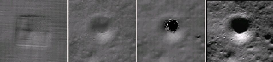
Fig. 11.3 An illustration of sfs. The images are, from left to right, the
hill-shaded initial guess DEM for SfS, the hill-shaded DEM obtained
from sfs, the “ground truth” DEM, and the first of the images
used in SfS map-projected onto the optimized DEM.
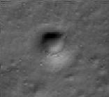
Fig. 11.4 An illustration of adding a curvature term to the SfS cost function, per Section 11.9.2. It can be seen that, compared to the earlier figure, the crater bottom is now curved, rather than flat, but more modeling is needed to ensure a seamless transition.
11.10. Large-scale SfS
SfS has been run successfully on a site close to the Lunar South Pole, at around 85.5 degrees South. Its size was 14336 x 11008 pixels, at 1 m/pixel. It used 814 LRO NAC images for bundle adjustment and 420 of those for SfS. The shadows on the ground were observed to make a full 360 degree loop. A seamless terrain was created (see the LPSC poster).
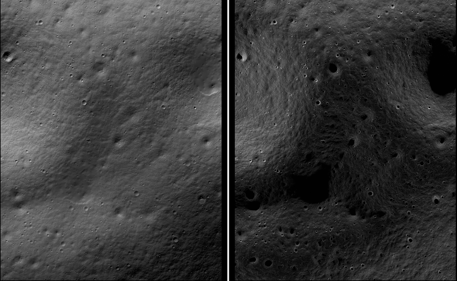
Fig. 11.5 A portion of a large-scale terrain produced with SfS showing a challenging area with very diverse illumination around some permanently-shadowed regions. Left: hillshaded SfS terrain. Right: max-lit mosaic. The quality of the produced terrain gracefully degrades as illumination gets worse.
11.10.1. Challenges
The challenges encountered were that the shadows were extensive and varied drastically from image to image, and some portions of the terrain showed up only in some images. All this made it difficult to register the images to each other and to the ground.
We solved this by doing bundle adjustment with a large number of images that were sorted by illumination conditions. We made sure that there exist images close to each other in the image list that overlap and have similar enough illumination, which resulted in all images being tied together.
The user is strongly cautioned that the difficulty of getting things right and figuring out what went wrong greatly increases with dataset complexity.
It is strongly suggested to first try SfS on a site of size perhaps 2000 x 2000 pixels, with a dozen carefully inspected images with slowly varying illumination, and having at least one stereo pair among them (Section 8.1) that can be used for alignment to the ground.
If happy with the results, more images can be added and the site size increased.
11.10.2. The initial terrain
A LOLA DEM was used as an initial guess terrain for SfS and as reference ground truth. A mosaic of several stereo DEMs with bundle-adjusted cameras can be used as well.
A Lunar South Pole 87-90 degree latitude DEM at 5 m/pixel is at:
Some lunar DEMs at 10 m/pixel and other resolutions, for latitude between 83 and 90 degrees South, are available at:
The site:
has LOLA DEMs at 5 m/pixel for a few locations.
A 20 meter/pixel LOLA product, which is rather low in resolution, but covers a significant portion of the South Pole, is available at:
http://imbrium.mit.edu/DATA/LOLA_GDR/POLAR/IMG/LDEM_80S_20M.IMG
http://imbrium.mit.edu/DATA/LOLA_GDR/POLAR/IMG/LDEM_80S_20M.LBL
11.10.3. Preprocessing the terrain
The higher-resolution DEMs mentioned above only need regridding.
The LDEM_80S_20M IMG and LBL files can be fetched with wget. Then, this
dataset should be converted to a .cub file as:
pds2isis from = LDEM_80S_20M.LBL to = ldem_80s_20m.cub
The heights for this DEM need to be multiplied by 0.5, per the information in
the LBL file. We do that with image_calc (Section 16.33):
image_calc -c "0.5*var_0" ldem_80s_20m.cub -o ldem_80s_20m_scale.tif
Resample the DEM to 1 m/pixel using gdalwarp (Section 16.25),
creating a DEM named ref_dem.tif:
gdalwarp -overwrite -r cubicspline -tr 1 1              \
  -co COMPRESSION=LZW -co TILED=yes -co INTERLEAVE=BAND \
  -co BLOCKXSIZE=256 -co BLOCKYSIZE=256                 \
  -te -7050.5 -10890.5 -1919.5 -5759.5                  \
  ldem_80s_20m_scale.tif ref_dem.tif
The values passed to -te are the bounds of the area of interest.
See a discussion about them below.
The DEM grid size should be not too different from the ground sample distance
(GSD) of the images, for optimal results. That one can be found with
mapproject (Section 16.41). For LRO NAC images, use 1 m / pixel.
It is suggested to use a stereographic projection. It should be a polar one, if around the poles, or otherwise centered at the area of interest. For example, set:
proj="+proj=stere +lat_0=-90 +lon_0=0 +R=1737400 +units=m +no_defs"
then run gdalwarp with the additional option -t_srs "$proj".
The interpolated DEM was created with bicubic spline interpolation, which is preferable to the default nearest neighbor interpolation, and it was saved internally using blocks of size 256 x 256, which ASP handles better than the GDAL default with each block as tall or wide as a row or column.
Inspect this DEM with stereo_gui (Section 16.72) in hillshade mode.
Any spikes or other artifacts should be blurred, such as by running:
dem_mosaic --dem-blur-sigma 2 ref_dem.tif -o ref_blur.tif
Any holes can also be filled with dem_mosaic (Section 16.20.2.9,
Section 16.20.2.8). A subsequent blur with a sigma of 2 pixels is
suggested (Section 16.20.2.6).
See Section 11.7.2 for how to create an initial DEM using stereo.
A stereo DEM can also be blended with the LOLA DEM using dem_mosaic
(after alignment, Section 11.10.9).
11.10.4. Terrain bounds
Later when we mapproject images onto this DEM, those will be computed at integer
multiples of the grid size, with each ground pixel centered at a grid point.
Given that the grid size is 1 m, the extent of those images as displayed by
gdalinfo will have a fractional value of 0.5.
The sfs_blend program will fail later unless the resampled initial
DEM also has this property, as it expects a one-to-one
correspondence between mapprojected images and the ground. Hence,
gdalwarp was used earlier with the -te option, with the bounds
having a fractional part of 0.5. Note that the bounds passed to
-te are in the order:
xmin, ymin, xmax, ymax
Ensure the min and max values are not swapped, as gdalwarp will not give a
warning if they are, but the resulting DEM will be incorrect.
The dem_mosaic program (Section 16.20) can be used to
automatically compute the bounds of a DEM or orthoimage and change
them to integer multiples of pixel size. It can be invoked, for
example, as:
dem_mosaic --tr 1 --tap input.tif -o output.tif
This will use bilinear interpolation.
11.10.5. Image selection and sorting by illumination
By far the hardest part of this exercise is choosing the images. We downloaded up to 1,400 of them, as described in Section 11.5, given the desired longitude-latitude bounds. The PDS .IMG files were converted to ISIS .cub cameras as in Section 11.7, and they were mapprojected onto the reference DEM, initially at a lower resolution to get a preview of things (Section 11.7.4).
It is very strongly recommended to use the CSM camera models instead of ISIS models (Section 11.6).
Inspection of a large number of images and choosing those that have
valid pixels in the area of interest can be very arduous. To make this
easier, we make use of the reporting facility of dem_mosaic
(Section 16.20) when invoked with the option
--block-max, with a large value of --block-size (larger than
the image size), and using the --t_projwin option to specify the
region of interest (in stereo_gui one can find this region by
selecting it with Control-Mouse).
When the mosaicking tool runs, the sum of pixels in the current region for each image will be printed to the screen. Images with a positive sum of pixels are likely to contribute to the desired region. Example:
dem_mosaic --block-max --block-size 10000 --threads 1   \
  --t_projwin -7050.500 -10890.500 -1919.500 -5759.500  \
  M*.map.lowres.tif -o tmp.tif | tee pixel_sum_list.txt
Eliminate the images that are not relevant to the area. Keeping them in impacts reliability and performance.
The obtained subset of images must be sorted by illumination conditions, that
is, the Sun azimuth, measured from true North. This angle is printed when
running sfs with the --query option on the .cub files. Here is an
example:
M114859732RE.cal.echo.cub       73.1771
M148012947LE.cal.echo.cub       75.9232
M147992619RE.cal.echo.cub       78.7806
M152979020RE.cal.echo.cub       96.895
M117241732LE.cal.echo.cub       97.9219
M152924707RE.cal.echo.cub       104.529
M150366876RE.cal.echo.cub       104.626
M152897611RE.cal.echo.cub       108.337
M152856903RE.cal.echo.cub       114.057
M140021445LE.cal.echo.cub       121.838
M157843789LE.cal.echo.cub       130.831
M157830228LE.cal.echo.cub       132.74
M157830228RE.cal.echo.cub       132.74
M157809893RE.cal.echo.cub       135.604
M139743255RE.cal.echo.cub       161.014
M139729686RE.cal.echo.cub       162.926
M139709342LE.cal.echo.cub       165.791
M139695762LE.cal.echo.cub       167.704
M142240314RE.cal.echo.cub       168.682
M142226765RE.cal.echo.cub       170.588
M142213197LE.cal.echo.cub       172.497
M132001536LE.cal.echo.cub       175.515
M103870068LE.cal.echo.cub       183.501
M103841430LE.cal.echo.cub       187.544
M142104686LE.cal.echo.cub       187.765
M162499044LE.cal.echo.cub       192.747
M162492261LE.cal.echo.cub       193.704
M162485477LE.cal.echo.cub       194.662
M162478694LE.cal.echo.cub       195.62
M103776992RE.cal.echo.cub       196.643
M103776992LE.cal.echo.cub       196.643
(the Sun azimuth is shown on the right, in degrees).
The primary reason why registration can fail later is illumination varying too drastically between nearby images, and not being able to find matching interest points. Hence, there must be sufficient images so that the illumination conditions over the entire site change slowly as one goes down the list.
A representative subset of the produced images can be found with the
program image_subset (Section 16.35). That tool must
be invoked once the images have been registered to each other and
to the ground, so later in the process (Section 11.10.13).
The paper [BMB+23] discusses how to automate the process of selecting images.
11.10.6. Incorporation of well-registered images
The approach outlined in the next sections consists of doing bundle adjustment, alignment, then refinement of bundle adjustment with ground constraints.
For the Lunar South Pole, a large set of well-registered cameras exists. Using
them requires running spiceinit with the provided kernels, followed
by creation of CSM cameras as usual.
In that case, consider first understanding the workflow below, then modify it as follows. In the first bundle adjustment, keep the subset of well-registered cameras for the given site fixed. Then, do not do alignment, but redo bundle adjustment with no fixed cameras, starting with the cameras from the first step. Lastly, run bundle adjustment with ground constraints as in the regular workflow.
The explanation is as follows. The well-registered cameras will help register the other cameras. Then alignment is not needed. However, a subsequent bundle adjustment with no fixed cameras will eliminate some minor registration issues in the well-registered cameras (which are known not to be perfect). The final bundle adjustment with the ground constraint reduces any vertical discrepancies.
11.10.7. Bundle adjustment
The parallel_bundle_adjust tool (Section 16.49)
is employed to co-register the images and correct camera errors. The
images must be, as mentioned earlier, ordered by Sun azimuth angle.
It is very important to have interest point matches that tie all images together. To make the determination of such matches more successful, the images were first mapprojected at 1 m/pixel (LRO NAC nominal resolution) to have them in the same perspective.
The mapprojected images must all be at the same resolution. Once images are mapprojected, the cameras used for that should not change, as that will result in incorrect results. See Section 12.2.4.3 for more details.
Create three lists, each being a plain text file with one file name on each line, having the input images (sorted by illumination), corresponding cameras (in .json or .cub format), and corresponding mapprojected images. The DEM used in mapprojection can be appended to the last list, but is optional (since the 1/2026 build) if it can be looked up in the geoheaders of the mapprojected images.
Run bundle adjustment:
parallel_bundle_adjust                           \
  --image-list image_list.txt                    \
  --camera-list camera_list.txt                  \
  --mapprojected-data-list mapprojected_list.txt \
  --processes 10                                 \
  --threads 8                                    \
  --ip-per-image 30000                           \
  --overlap-limit 100                            \
  --num-iterations 100                           \
  --num-passes 2                                 \
  --min-matches 1                                \
  --max-pairwise-matches 2000                    \
  --camera-weight 0                              \
  --robust-threshold 2                           \
  --tri-weight 0.05                              \
  --tri-robust-threshold 0.05                    \
  --remove-outliers-params "75.0 3.0 100 100"    \
  --save-intermediate-cameras                    \
  --match-first-to-last                          \
  --forced-triangulation-distance 100000         \
  --min-triangulation-angle 1e-10                \
  --datum D_MOON                                 \
  --nodes-list <list of computing nodes>         \
  -o ba/run
The option --overlap-limit needs a large value, but the process can take a
very long time. The --auto-overlap-params option can help determine which
images overlap.
The key reason for failure in this process is images not being matched to enough relevant consecutive images, or simply not having enough such images to start with.
Here more bundle adjustment iterations are desirable,
but this step takes too long. A large --ip-per-image can make a
difference in images with rather different illumination
conditions but it can also slow down the process a lot. Note that the
value of --max-pairwise-matches was set to 2000. That should
create enough matches among any two images. A higher value
here will make bundle adjustment run slower and use more memory.
Towards the poles the Sun may describe a full loop in the sky, and
hence the earliest images (sorted by Sun azimuth angle) may become
similar to the latest ones. That is the reason above we used the
option --match-first-to-last.
If having an estimate of how accurate initial camera positions are, the option
--camera-position-uncertainty is suggested. If this uncertainty is too
small, it can prevent convergence. For LRO NAC, perhaps 100 - 500 m is a good
value. See also Section 16.5.11.2.
Note that this invocation may run for over a day, and may be necessary
for good convergence. If the process gets interrupted, or the user
gives up on waiting, the adjustments obtained so far can still be
usable, if invoking bundle adjustment, as above, with
--save-intermediate-cameras.
As before, using the CSM model can result in much-improved performance.
Here we used --camera-weight 0 and --robust-threshold 2 to
give cameras which start far from the solution more chances to
converge. We are very generous with outlier filtering in the option
--remove-outliers-params. That will ensure that in case the
solution did not fully converge, valid matches with large
reprojection error are not thrown out as outliers.
A large value of --processes can result in running out of memory.
11.10.8. Validation of bundle adjustment
The file:
ba/run-final_residuals_stats.txt
should be examined. The median reprojection error per camera must be at most 1-2
pixels (the mean error could be larger). If that is not the case, bundle
adjustment failed to converge. To help it, consider doing a preliminary step of
bundle adjustment with --robust-threshold 5 to force the larger errors to go
down, and then do a second invocation to refine the cameras with
--robust-threshold 2 as earlier.
In the second invocation, either use the original cameras and with the option
--input-adjustments-prefix, pointing to the latest adjustments, or use the
latest optimized cameras, if in CSM format.
Reuse the match files with the option --match-files-prefix.
It is best to avoid throwing out images at this stage. More images mean a higher chance that the images will be tied together. The images that have a zero count in the stats file can be thrown out.
11.10.9. Alignment to the ground
A very critical part of the process is to move from the coordinate
system of the cameras to the coordinate system of the initial guess
terrain in ref_dem.tif. The only reliable approach for this is to
create a terrain model using stereo with some of the images and
bundle-adjusted cameras produced so far, align that one to ref_dem.tif,
and then apply this alignment to the cameras.
With LRO NAC images, stereo pairs may be hard to find. In addition, after the earlier step of bundle adjustment the images may already be within 10-30 meters horizontally relative to the reference LOLA DEM, as validated by mapprojection.
If it looks that the alignment is already in the ballpark, and it is tricky to find stereo pairs, or the attempt at alignment fails, consider skipping this step.
The produced SfS DEM will likely need additional alignment in either case (Section 11.10.14).
Examine the file having the stereo convergence angles for each pair of images as produced by bundle adjustment (Section 16.5.11.4). Eliminate those with a convergence angle of under 10 degrees or so, and sort the rest in decreasing number of matches (if not enough pairs left, can decrease this angle to 3 - 5 degrees).
Produce 30 - 100 stereo DEMs from the stereo pairs with non-small convergence angles. These must cover well the full site, even if there are missing areas in between. This helps with consistent alignment.
It is very important that the camera adjustments created so far are used in
stereo, by passing them via --bundle-adjust-prefix. Or, with CSM cameras,
can use the latest optimized cameras instead, without the
--bundle-adjust-prefix option. Stereo with mapprojected images is preferable
(Section 6.1.7).
So, the stereo command can look as follows:
parallel_stereo A.map.tif B.map.tif \
  ba/run-A.adjusted_state.json      \
  ba/run-B.adjusted_state.json      \
  --stereo-algorithm asp_mgm        \
  --subpixel-mode 9                 \
  run_stereo/run                    \
  ref_dem.tif
Here, ref_dem.tif is the DEM used for mapprojection. Note that the
mapprojected images won’t fully agree with the DEM or each other yet, as they
are not registered to the DEM, but stereo should still run fine.
When invoking point2dem on the resulting point clouds, use the same
projection (--t_srs) as in the reference terrain and a grid size (--tr)
of 1 meter. Inspect the triangulation error (Section 16.56). Ideally its
average should not be more than 1 meter.
The created DEMs can be mosaicked with dem_mosaic
(Section 16.20) as:
dem_mosaic -o stereo_mosaic.tif --dem-list stereo_dem_list.txt
It is strongly suggested to use the geodiff program (Section 16.26) to
inspect how well the individual DEMs agree with their mosaic. This can help
catch problems early. If most DEMs agree well with the mosaic, but some are way
off, this may need investigation, or the bad ones can be thrown out, and the
mosaic redone.
Overlay and inspect the produced stereo DEM mosaic and the reference DEM in
stereo_gui.
Align the mosaicked DEM to the initial LOLA terrain in ref_dem.tif
using pc_align (Section 16.53):
pc_align --max-displacement 500           \
  stereo_mosaic.tif ref_dem.tif           \
  --save-inv-transformed-reference-points \
  -o run_align/run
The output 50th error percentile of smallest errors as printed by this tool should be under 1-5 meters, and ideally less. Otherwise likely something is not right, and the registration of images may fail later.
The pc_align tool can be quite sensitive to the
--max-displacement value. It should be somewhat larger than the
total estimated translation (horizontal + vertical) among the two
datasets. The option --compute-translation-only may be necessary
if pc_align introduces a bogus rotation.
The resulting transformed cloud run_align/run-trans_reference.tif
needs to be regridded with point2dem with the same projection
and grid size as before.
This DEM should be hillshaded (Section 16.28) and overlaid on top of the LOLA DEM to see if there is any noticeable shift, which would be a sign of alignment not being successful.
If no luck, and visually the misalignment looks small horizontally, alignment could be skipped, for now, and one could continue with the next step, of using a DEM constraint, to fix vertical alignment issues. After that, perhaps alignment will work better.
The geodiff tool should be used to examine any discrepancy among the two
(Section 16.26), followed by colormap (Section 16.14) and
inspection in stereo_gui.
If happy with the results, the alignment transform can be applied to the cameras. With CSM cameras, that goes as follows:
bundle_adjust                                             \
  --image-list ba/run-image_list.txt                      \
  --camera-list ba/run-camera_list.txt                    \
  --initial-transform run_align/run-inverse-transform.txt \
  --apply-initial-transform-only                          \
  -o ba_align/run
It is very important to note that we used above
run-inverse-transform.txt, which goes from the stereo DEM
coordinate system to the LOLA one. This is discussed in detail in
Section 16.53.14. We used the latest optimized cameras
in the ba directory.
It is suggested to mapproject the images using the obtained
bundle-adjusted cameras in ba_align/run onto ref_dem.tif, and
check for alignment errors in stereo_gui by overlaying the images
using georeference information. Small errors (under 5-10 pixels) are
likely fine and will be corrected at the next step.
If the images are too many, inspect at least a dozen of them. The report file introduced at the next step will help with a large number of images.
The following command can be used to quickly overlay a few dozen mapprojected images:
stereo_gui --hide-all --single-window --use-georef $(cat list.txt)
Then individual images can be toggled on and off.
11.10.10. Registration refinement
If the images mapproject reasonably well onto the reference DEM, with no shift across the board, but there are still some registration errors, one can refine the cameras using the reference terrain as a constraint in bundle adjustment (Section 12.2.1.3):
bundle_adjust                                 \
  --image-list ba_align/run-image_list.txt    \
  --camera-list ba_align/run-camera_list.txt  \
  --match-files-prefix ba/run                 \
  --max-pairwise-matches 2000                 \
  --match-first-to-last                       \
  --min-matches 1                             \
  --skip-matching                             \
  --num-iterations 100                        \
  --num-passes 2                              \
  --camera-weight 0                           \
  --save-intermediate-cameras                 \
  --heights-from-dem ref_dem.tif              \
  --heights-from-dem-uncertainty 20.0         \
  --mapproj-dem ref_dem.tif                   \
  --forced-triangulation-distance 100000      \
  --min-triangulation-angle 1e-10             \
  --remove-outliers-params "75.0 3.0 100 100" \
  --parameter-tolerance 1e-20                 \
  --threads 20                                \
  -o ba_align_ref/run
Note how we use the match files with the original ba/run prefix,
and also use --skip-matching to save time by not recomputing
them. But the cameras come from ba_align/run, as the
ones with the ba/run prefix are before alignment.
We used the CSM cameras (Section 11.6).
The option --mapproj-dem is very helpful for identifying
misregistered images (see below).
The value used for --heights-from-dem-uncertainty can be larger, such as
100, if it is believed that the stereo DEM mosaic produced so far is too
different from LOLA. See also Section 12.2.1.3.
The switch --save-intermediate-cameras is helpful, as before, if
desired to stop if things take too long.
11.10.11. Validation of registration
Mapproject the input images with the latest aligned cameras:
mapproject --tr 1.0                          \
  ref_dem.tif                                \
  image.cub                                  \
  ba_align_ref/run*image.adjusted_state.json \
  image.align.map.tif
Above, the correct camera for the given image should be picked up from the latest bundle-adjusted and aligned camera directory.
These resulting mapprojected images can be overlaid in stereo_gui with
georeference information and checked for misregistration. A maximally-lit mosaic
can be created with the command:
dem_mosaic --max -o max_lit.tif *.align.map.tif
Misregistered images will create ghosting in this mosaic.
Given, for example, a few hundred input images, it is very time-consuming to do pairwise inspections to find the misaligned images. Bundle adjustment created a report file with the name:
ba_align_ref/run-mapproj_match_offset_stats.txt
which greatly simplifies this job. This file shows how much each mapprojected image disagrees with the rest, in meters. See Section 16.5.11.10 for details.
Images with low count in this report can be thrown out. If the 85th percentile of registration errors for an image is over 1.5 meters (assuming a 1 meter ground resolution), it likely registered badly. Those can be deprioritized.
The more images are eliminated, the more one risks loss of coverage. It is suggested to sort the images in increasing order of 85th percentile of misregistration error, and create a few candidate sets, with each set having a different threshold for what is considered an acceptable registration error. For example, use cutoffs of 1.25 m, 1.5 m, 1.75 m.
Create the maximally lit mosaic for each of these and overlay them
in stereo_gui. Inspect them carefully. Choose the set which
does not sacrifice coverage and has a small amount of misregistration.
Some images with a larger registration error could be added after
careful inspection, to increase the coverage.
The images with a high 95th error percentile (say over 2 meters) should be overlaid on top of this maximally lit mosaic and removed if they show obvious misregistration.
See also the earlier section of validation of bundle adjustment (Section 11.10.8). That one discusses a report file that measures the errors in the pixel space rather than on the ground.
Further refinement and re-validation can be done after solving for jitter, but this is a more advanced topic (Section 11.10.22).
11.10.12. Handling failure
If the maximally lit mosaic has registration errors, most frequent causes are:
Images were not sorted by illumination in bundle adjustment.
There are not enough images of intermediate illumination to tie the data together.
The interest point matches are inaccurate (locking onto moving shadows).
The value of
--overlap-limitwas too small.Horizontal or vertical alignment failed.
Ensure that the recipe in Section 11.10 was followed carefully. Further strategies:
See if many mapprojected images are misregistered with the DEM. If yes, bundle adjustment and/or alignment failed and needs to be redone or refined.
Crop all mapprojected images produced with bundle-adjusted cameras to a small site, and overlay them while sorted by illumination (solar azimuth angle). See for which images the registration failure occurs.
Inspect the match files for unprojected images (
.matchandclean.match) instereo_gui(Section 16.72.9.2). Perhaps there were not enough matches or too many of them were thrown out as outliers.Fallback to a smaller subset of images which is self-consistent, even if losing coverage that way. Can be guided for this by the report files (Section 11.10.11, Section 11.10.8).
See if more images can be added with intermediate illumination conditions and to increase coverage.
If a well-aligned SfS terrain is produced with a subset of the images, consider
doing the same for a subset of the remaining ones. The second SfS terrain can be
aligned to the first one on a clip where they both produce good results, with
pc_align with correlation-based alignment (Section 16.53.3.5) and the option
--initial-transform-from-hillshading translation. This alignment can be
applied to the full second terrain.
Alternatively, max-lit mosaics for the subsets could be correlated (Section 16.17), and the produced disparity could be used for image (Section 16.32) and terrain alignment (Section 16.53.3.5).
If the alignment is successful, apply it to the second set of cameras as well
(Section 16.53.14), and then tighten the vertical alignment for the second
set with bundle_adjust with the option --heights-from-dem, as above. Then,
joint SfS for the union of the two sets should work.
If no luck, break up a large site into 4 quadrants with overlap, eliminate all images not having good pixels in a given quadrant, and create a solution for each. Any match file should however have features in the full site, for reuse later.
If the resulting subsets of bundle-adjusted cameras are individually
self-consistent and consistent with the ground, do a combined bundle adjustment
using the union of all sets of match files, by copying them to a single
directory, with --overlap-limit set to 0 to use all match files. Ensure that
each match file extends over the full region in that case.
The image_align program (Section 16.32) was reported to be of help
in co-registering images. Note however that failure of registration is almost
surely because not all images are connected together using match points, or the
images are consistent with each other but not with the ground.
Note that interest point matches produced from stereo (Section 12.2.4.2) are less sensitive to illumination changes, but that process is quite slow and does not scale for a large number of pairwise matches.
11.10.13. Running SfS in parallel
Next, SfS follows, using parallel_sfs (Section 16.50):
parallel_sfs -i ref_dem.tif                      \
  --nodes-list nodes_list.txt                    \
  --processes 6                                  \
  --threads 8                                    \
  --tile-size 200                                \
  --padding 50                                   \
  --image-list ba_align_ref/run-image_list.txt   \
  --camera-list ba_align_ref/run-camera_list.txt \
  --shadow-threshold 0.005                       \
  --use-approx-camera-models                     \
  --crop-input-images                            \
  --blending-dist 10                             \
  --min-blend-size 50                            \
  --allow-borderline-data                        \
  --low-light-threshold 0.03                     \
  --smoothness-weight 0.08                       \
  --initial-dem-constraint-weight 0.0025         \
  --reflectance-type 1                           \
  --max-iterations 5                             \
  --save-sparingly                               \
  -o sfs/run
For this step not all images need to be used, just a representative enough subset. Normally, having two or three sufficiently different illumination conditions at each location is good enough, ideally with the shadows from one image being roughly perpendicular to shadows from other images.
A representative subset of the produced images can be found with the
program image_subset (Section 16.35). Invoke that program
with low-resolution versions of the mapprojected co-registered input
images. That program’s page has more details.
SfS should work fine with a few hundred input images, but it can be slow.
It is best to avoid images with very low illumination angles as those can result in artifacts in the produced SfS terrain.
The first step that will happen, when this program is launched, is computing the
image exposures, and, if applicable, the initial haze values and albedo. See the
option --estimate-exposure-haze-albedo in Section 16.67 for more details.
Then the computed exposures (also haze and albedo, if applicable) are passed to
each tile that is run in parallel, via --image-exposures-prefix (and, if
applicable, --haze-prefix, --input-albedo). All these are further
optimized per tile if --float-exposure, --float-haze, and/or
--float-albedo are used.
The option --allow-borderline-data improves the level of detail
close to permanently shadowed areas. See Section 11.9.1.
It was found empirically that a shadow threshold of 0.005 was good
enough. It is also possible to specify individual shadow thresholds
if desired, via --custom-shadow-threshold-list. This may be useful
for images having diffuse shadows cast from elevated areas that are
far-off. For those, the threshold may need to be raised to as much as
0.01.
The value of --initial-dem-constraint-weight may need to be increased
somewhat if the resulting SfS terrain differs too much from the initial LOLA
terrain, or if a tiling pattern is seen. The geodiff program
(Section 16.26) can help evaluate the difference.
Use a larger --blending-dist if the produced terrain has visible artifacts
around shadow regions which do not go away after increasing the shadow
thresholds. To get more seamless results around small shadowed craters reduce
the value of --min-blend-size. This can result in more erosion.
See Section 11.10.17 for fixing seams in low-light areas.
The option --use-approx-camera-models is not necessary with CSM
cameras.
One should experiment with floating the albedo (option
--float-albedo) if noticeable albedo variations are seen in the
images. See Section 11.8 for a longer discussion. It is suggested
to run SfS without this flag first and inspect the results.
When it comes to selecting the number of nodes to use, it is good to notice how
many tiles the parallel_sfs program produces (the tool prints that), as a
process will be launched for each tile. Since above it is chosen to run 5-10
processes on each node, the number of nodes can be a fraction of the number of
tiles over number of processes. One should examine how much memory and CPU these
processes use and adjust these numbers accordingly.
See Section 11.9.2 for a potential solution for SfS producing flat crater bottoms where there is no illumination to guide the solver. See Section 11.9.1 for a very preliminary solution for how one can try to improve very low-lit areas (it only works on manually selected clips and 1-3 images for each clip).
See an illustration of the produced terrain in Fig. 11.5.
11.10.14. Inspection and refinement
The obtained shape-from-shading terrain should be studied carefully to see if it
shows any systematic shift or rotation compared to the initial LOLA gridded
terrain. For that, the SfS terrain can be overlaid as a hillshaded
(Section 16.28) image on top of the initial terrain in stereo_gui, in
georeference mode, and the SfS terrain can be toggled on and off.
11.10.14.1. Measurement of misalignment
Misalignment can be measured quantitatively by hillshading the gridded LOLA and SfS terrain and doing stereo correlation. This goes as follows.
Hillshade both DEMs:
hillshade -e 10 ref_dem.tif -o ref_dem_hill.tif
hillshade -e 10 sfs_dem.tif -o sfs_dem_hill.tif
It is assumed as before that these two DEMs have precisely the same projection,
grid size and extent. Consider adjusting the elevation (-e) parameter and
also the azimuth (-a) parameter to produce well-lit images with good range
of intensities that fill most of the 0 to 255 range.
If some areas appear saturated or too much in shadow, consider a hillshade command along the lines of:
gdaldem hillshade -multidirectional -compute_edges -alt 20 \
  dem.tif dem_hill.tif
Run stereo in correlator mode (Section 16.17):
parallel_stereo               \
  --correlator-mode           \
  --stereo-algorithm asp_mgm  \
  --corr-kernel 9 9           \
  --ip-per-image 40000        \
  --subpixel-mode 9           \
  --corr-search -25 -25 25 25 \
  --nodes-list nodes_list.txt \
  sfs_dem_hill.tif            \
  ref_dem_hill.tif            \
  sfs_ref_corr/run
The search range in --corr-search is determined by the expected amount of
misalignment (Section 14.4.2).
Here, the SfS DEM is intentionally specified as the first input, as that is needed by subsequent logic.
The produced F.tif disparity can be split into bands while masking no-data
values (Section 16.33.1.10) and viewed with stereo_gui
(Section 16.72.5) as:
stereo_gui --colorbar              \
  --min -10 --max 10               \
  sfs_ref_corr/run-F_b1_nodata.tif \
  sfs_ref_corr/run-F_b2_nodata.tif
It is very important to confirm that the visually-observed shifts agree with the disparities shown by this plot.
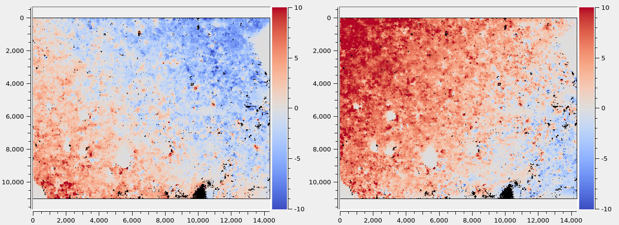
Fig. 11.6 Colorized horizontal and vertical disparities from the SfS DEM to the LOLA DEM. There exists a horizontal misalignment of 5 pixels in the upper-right corner (left plot), and a vertical misalignment of 10 pixels in the upper-left corner (right plot).
A sample plot of such disparities is shown in Fig. 11.6. It can be seen
that here the misregistration is large and non-uniform. In this case, the only
reliable solution for repair is to make use of custom GCP produced with
dem2gcp as seen in the next section. A simpler recipe for correcting a shift
or rotation only with pc_align is shown further down.
11.10.14.2. GCP-based refinement
The dem2gcp program (Section 16.18) will take as input this disparity
and move each ground point produced by triangulation of interest point matches
from the “warped” location on the SfS DEM to the correct location on the LOLA
DEM, forming ground control points (Section 16.5.9).
This invocation requires a build of ASP as of 2025/11 or later (Section 2.1).
dem2gcp                                            \
  --warped-dem sfs_dem.tif                         \
  --ref-dem ref_dem.tif                            \
  --warped-to-ref-disparity sfs_ref_corr/run-F.tif \
  --image-list ba_align_ref/run-image_list.txt     \
  --camera-list ba_align_ref/run-camera_list.txt   \
  --clean-match-files-prefix ba/run                \
  --max-pairwise-matches 5000                      \
  --gcp-sigma 1.0                                  \
  --max-num-gcp 2000000                            \
  --output-gcp sfs_ref_corr/run.gcp
The value of --gcp-sigma should be on the order of the ground sample distance
(in meters), to ensure that the GCP constraint is strong enough.
This program can be sensitive to outliers, so the clean matches above should be
produced with bundle adjustment with a value of --remove-outliers-params
that removes outliers with reprojection error more than 5-10 pixels or so.
The resulting GCP file can be passed to bundle_adjust together with the
images and latest cameras, such as in Section 11.10.10.
Care must be taken that these GCP do not conflict with triangulated points in
bundle adjustment, with or without the --heights-from-dem option. See
Section 16.18.5.
Then, SfS must be rerun with the new cameras. Misalignment can be evaluated as before.
If the horizontal misregistration got fixed, but some local inconsistencies in
the max-lit mosaic are observed, a subsequent pass of bundle adjustment with
latest cameras, without GCP this time, with the --heights-from-dem option as
usual, can repair this.
The created SfS terrain can be employed to improve the registration of any problematic images (Section 11.10.19).
11.10.14.3. Refinement based on a rigid transform
If the misalignment looks as if produced by a rigid transform, one can try alignment based on dense correlation of hillshaded images (Section 16.53.3.5). This requires that the correlation be run with the inputs in reverse order from the above, so the first input would be the reference LOLA DEM.
Alternatively, one can do sparse features-based alignment
(Section 16.53.3.4). This works better on lower-resolution versions of the
inputs, when the high-frequency discrepancies do not confuse the alignment, so,
for example, at 1/4 or 1/8 resolution of the DEMs, as created with stereo_gui:
pc_align --initial-transform-from-hillshading rigid    \
  ref_dem_sub4.tif sfs_dem_sub4.tif -o align_sub4/run  \
  --num-iterations 0 --max-displacement -1
In either case, the alignment transform can then be applied to the full SfS DEM (Section 16.53.6):
pc_align --initial-transform align_sub4/run-transform.txt      \
  ref_dem.tif sfs_dem.tif -o align/run --num-iterations 0      \
  --max-displacement -1 --save-transformed-source-points       \
  --max-num-reference-points 1000 --max-num-source-points 1000
The number of points being used is not important since we will just apply the alignment and transform the full DEM.
The aligned SfS DEM can be created from the obtained transformed cloud as:
point2dem --tr 1 --search-radius-factor 2 --t_srs projection_str \
  align/run-trans_source.tif
Here, the projection string should be the same one as in the reference
LOLA DEM named ref_dem.tif. It can be found by invoking:
gdalinfo -proj4 ref_dem.tif
and looking for the value of the PROJ field.
The alignment transform should be applied to the cameras (Section 16.53.14), then bundle adjustment with a terrain constraint should be redone as in Section 11.10.10.
Lastly, the SfS DEM must be regenerated with the new cameras.
Ideally, after all this, there should be no systematic offset between the SfS terrain and the reference LOLA terrain.
11.10.14.4. Image-based refinement
Another approach is to find the stereo disparity from the hillshaded SfS DEM to
the hillshaded reference DEM (at 1/4th the resolution) with parallel_stereo
--correlator-mode, then invoke image_align (Section 16.32) on the
disparity. It appears that the stereo correlation works better if the first
cloud is the SfS DEM, as it has more detail. This can produce an alignment
transform (Section 16.32.6) that can be passed in to
pc_align with zero iterations to align the SfS DEM to the reference DEM
(Section 16.53.6).
11.10.14.5. Manual alignment
If these approaches fail to remove the visually noticeable displacement
between the SfS and LOLA terrain, one can try to nudge the SfS terrain
manually, by using pc_align as:
pc_align --initial-ned-translation                             \
  "north_shift east_shift down_shift"                          \
  ref_dem.tif sfs_dem.tif -o align/run --num-iterations 0      \
  --max-displacement -1 --save-transformed-source-points       \
  --max-num-reference-points 1000 --max-num-source-points 1000
Here, the value of down_shift should be 0, as we attempt a horizontal shift. For
the others, one may try some values and observe their effect in moving the
SfS terrain to the desired place.
The transform obtained by using these numbers will be saved in
align/run-transform.txt (while being converted from the local
North-East-Down coordinates to ECEF) and can be used to transform the cameras
to bring them in closer alignment with the reference terrain.
If a manual rotation nudge is necessary, use pc_align with
--initial-rotation-angle.
The transformed cloud then needs to be regridded with point2dem
as before.
In all cases the SfS DEM must be regenerated with the aligned cameras.
11.10.15. Comparison with initial terrain
The geodiff tool can be deployed to see how the SfS DEM compares
to the initial guess or to the raw ungridded LOLA measurements.
One can use the --absolute option for this tool and then invoke
colormap to colorize the difference map. By and large, the SfS
DEM should not differ from the reference DEM by more than 1-2 meters.
It is also suggested to produce a maximally-lit mosaic, as in Section 11.10.11. This should not look too different if projecting on the initial guess DEM or on the refined one created with SfS.
11.10.16. Handling issues in the SfS result
Misregistration errors between the images can result in craters or other features being duplicated in the SfS terrain. Then, registration must be redone as discussed in the earlier sections.
If in some low-light locations the SfS DEM has seams, see Section 11.10.17.
Artifacts around permanently shadowed areas can be fixed with sfs_blend
(Section 16.68).
See Section 11.9.1 for how to increase the coverage in areas with very low illumination.
If the SfS DEM has localized defects, those can be fixed in a small region and
then blended in. For example, a clip around the defect, perhaps of dimensions
400 pixels or larger, can be cut from the input DEM. If that clip has noise
which affects the final SfS result, it can be blurred with dem_mosaic, using
for example, --dem-blur-sigma 2 (or a larger sigma value). Then one can try
to run parallel_sfs on just this clip, and if needed, vary some of the SfS
parameters or exclude some images.
If happy enough with the result, this small SfS clip can be blended back to the
larger SfS DEM with dem_mosaic as:
dem_mosaic --priority-blending-length 75         \
  small_sfs.tif large_sfs.tif -o merged_sfs.tif
Inspect the resulting hillshaded DEM to ensure this did not result in blending artifacts.
11.10.17. Fixing seams in the SfS terrain
Images with partially shadowed areas can result in seams in the SfS hillshaded DEM. The best available approach for fixing these problems starts by setting a threshold for such semi-shadowed pixels. Pixels with values between this and the shadow threshold will be given less weight, in inverse proportion to the discrepancy between the observed and simulated pixel value.
This weight can be raised to a certain power to make this attenuation effect stronger, and the resulting weight image can be blurred somewhat to reduce any discontinuities.
Pixels for which no other images have higher values at the given ground location are excluded from this process, to avoid unnecessary erosion. (However, the blur operation on the weights, per above, may still result in some erosion.)
This approach is available with a build from 2025/11 or later (Section 2.1).
After extensive experimentation, it was validated that this option works well
when enabled for a full run, not just for clips that show seams. If not desired,
remove the --low-light-threshold option from the parallel_sfs invocation
(Section 11.10.13).
To enable this approach, the option --allow-borderline-data is assumed
(Section 11.9.1). Then, the following additional options are needed:
--low-light-threshold 0.03   \
--low-light-weight-power 4.0 \
--low-light-blur-sigma 3.0
The value of --low-light-threshold should be chosen based on the specific
dataset. For LRO NAC, where the shadow threshold is around 0.005, a value of
0.03 was observed to work well.
The full documentation for these options is Section 16.67.
How to blend in repaired clips is discussed in Section 11.10.16.
11.10.18. Blending the SfS result with the initial terrain
After computing a satisfactory SfS DEM, it can be processed to replace the values in the permanently shadowed areas with values from the LOLA reference DEM, with a transition region.
This process will fail unless the SfS DEM and the LOLA DEM have the same grid. How to prepare the initial terrain is described in Section 11.10.2, and more details about bounds are in Section 11.10.4. A workaround is suggested later in this section.
The blending can be done as:
sfs_blend --lola-dem lola_dem.tif --sfs-dem sfs_dem.tif      \
  --max-lit-image-mosaic max_lit.tif --image-threshold 0.005 \
  --lit-blend-length 25 --shadow-blend-length 5              \
  --min-blend-size 25 --weight-blur-sigma 5                  \
  --output-dem sfs_blend.tif --output-weight sfs_weight.tif
Here, the inputs are the LOLA and SfS DEMs, the maximally lit mosaic provided as before, the shadow threshold (the same value as in invoking SfS should be used). These are expected to have precisely the same extent, projection, and resolution.
The outputs are the blended DEM as described earlier, and the weight
which tells how much the SfS DEM contributed to the blended DEM. That
weight equals to 1 where only the SfS DEM was used, is between 0 and 1
in the transition region between the lit and shadowed areas, which is
determined by the values of the --lit-blend-length and
--shadow-blend-length parameters (it grows somewhat depending on
the value of --weight-blur-sigma), and is 0 where only the LOLA
values contribute to the solution. The weight function is the
truncated signed Euclidean distance to the lit boundary, scaled to have
values between 0 and 1, then blurred with a Gaussian kernel with the
above-mentioned sigma. No blending happens for shadowed regions of
dimensions less than --min-blend-size, where the SfS DEM is
kept. See Section 16.68 for more details.
If sfs_blend fails due to the grids not matching, it is suggested that the
input LOLA terrain be prepared with gdalwarp -te <corners> as described in
Section 11.10.2, and then the SfS terrain be regenerated starting
with this terrain, with any desired transform applied to the cameras before
parallel_sfs is rerun, and then the extent of the LOLA and SfS terrains will
agree.
Or, the SfS terrain which exists so far (sfs_dem.tif), the LOLA terrain
(lola_dem.tif), and the maximally lit mosaic (max_lit.tif) can all be
resampled to the same grid with gdalwarp with the --te and -r
cubicspline options, or with dem_mosaic --tap, before invoking
sfs_blend.
11.10.19. Post-SfS registration
This section discusses how to use a produced SfS terrain to measure and repair any misregistration of input images. It is assumed that this SfS terrain is well-registered to the reference DEM (e.g., from LOLA), as validated in Section 11.10.14.
Image misregistration can arise from the fact that interest point matching can be inaccurate for images with diverse illumination conditions, as discussed in Section 11.10.12.
We make use of the observation that given a raw (measured) image and corresponding camera, a simulated image with the same view and illumination, produced with the SfS terrain, will look very similar to the raw mapprojected image, apart from some shift or rotation. This discrepancy can be measured and corrected, bringing the images in better registration with the SfS terrain.
This process is done for each image individually. The resulting improved cameras could be used to create a refined SfS terrain.
To define some notation, let sfs_dem.tif be the final SfS DEM, image.cub
be the input raw image, and camera.json be the best-registered camera
available for this image.
Mapproject the raw image onto the SfS DEM with this camera, producing
image_map.tif:
mapproject    \
  --tr 1.0    \
  sfs_dem.tif \
  image.cub   \
  camera.json \
  image_map.tif
Create the simulated orthoimage (this requires a build from 2025/12 or later, Section 2.1):
sfs -i sfs_dem.tif              \
    --save-sim-intensity-only   \
    image.cub                   \
    camera.json                 \
    --ref-map image_map.tif     \
    -o run/image
This will write run/image-camera-sim-intensity.tif. Ensure the name of this
file is unique for each input image.
Inspect the measured and simulated orthoimages. They should be very similar,
apart from any misregistration. The image_align tool (Section 16.32)
can find the transform that aligns the measured image to the simulated one.
Note that the simulated image is the reference, and is specified first.
image_align                            \
    --ip-detect-method 0               \
    --inlier-threshold 50              \
    --ip-per-tile 2500                 \
    --ip-per-image 0                   \
    --alignment-transform translation  \
    run/image-camera-sim-intensity.tif \
    image_map.tif                      \
    --output-prefix align/run          \
    -o aligned_image.tif
This transform will be saved to a file. It will also be printed to standard
output and recorded in the log file after the line Alignment transform (in
pixels). It is suggested to also check the number of interest point matches
inliers in the log file, as that can be a proxy for how accurate the computed
transform is.
For a more complex misregistration, one can try a rigid transform. This is a
bit harder to interpret.
The gcp_gen program (Section 16.24) can create ground control points
(GCP, Section 16.5.9). These GCP will tie pixel locations in the original raw
image to 3D locations on the SfS DEM.
gcp_gen                                              \
    --ip-detect-method 0                             \
    --inlier-threshold 50                            \
    --ip-per-image 0                                 \
    --ip-per-tile 2500                               \
    --gcp-sigma 1.0                                  \
    --camera-image image.cub                         \
    --mapproj-image image_map.tif                    \
    --ortho-image run/image-camera-sim-intensity.tif \
    --dem sfs_dem.tif                                \
    --output-prefix gcp_gen/run                      \
    -o image_gcp.gcp
A GCP sigma of 1.0 meter is reasonable if the DEM resolution is 1 m/pixel.
The newly created GCP file is used with bundle_adjust
(Section 16.5) to refine the camera model for the input image.
bundle_adjust     \
    image.cub     \
    camera.json   \
    image_gcp.gcp \
    -o ba_gcp/run
This will produce an updated camera model named ba_gcp/run-image.json.
To validate the correction, mapproject the input image with the newly aligned camera:
mapproject --tr 1.0     \
  sfs_dem.tif           \
  image.cub             \
  ba_gcp/run-image.json \
  image_aligned.tif
The resulting orthoimage should show better agreement with the SfS DEM, with the simulated image, and with other similarly aligned images. This process can be repeated for all input images.
11.10.20. Creation of mask of SfS pixels
The SfS DEM used the information from images where the ground was lit, so above the shadow threshold. In the shadowed areas just the smoothness constraint and initial DEM constraint were used. To create the mask of such lit pixels, with value of 1 where lit and 0 where unlit, use the maximally-lit mosaic found earlier, and run:
thresh=0.005
image_calc -c "sign(max(var_0, $thresh) - $thresh)" \
  max_lit.tif -o sfs_mask.tif
Here, the shadow threshold used during SfS should be used, separating lit and unlit pixels.
11.10.21. SfS height uncertainty map
The recommended approach for assessing the quality of the SfS result is to compute the variance for each DEM pixel (available in ASP 3.6.0 or later).
The square root of the variance is the standard deviation, a relative measure of DEM height uncertainty. This feature is experimental: the values are uncalibrated and they do not represent real elevation uncertainties in meters.
Use the --save-variances option (Section 16.67.6) with parallel_sfs
(Section 11.10.13). The resulting output file is described in
Section 16.67.5.
The variance is computed from the diagonal of the covariance matrix of the optimized parameters, using the Ceres Covariance Estimation method.
The --save-covariances option (Section 16.67.6), available in build 2026/2
or later (Section 2.1), saves the covariance between each DEM pixel and
four nearby neighbors, at row and column offsets (0, +2), (+1, -1), (+1, +1),
and (+2, 0). These are the pixel pairs that enter the central-difference
(three-point) slope, so with the variance they let the height uncertainty be
propagated into a slope uncertainty, and they help reveal the spatial
correlation of errors. See Section 16.67.5 for the output files.
Previously, the option --estimate-height-errors was employed, with a
different implementation. This is now obsolete. See Section 16.67.6 for
details.
A useful exercise is to run SfS with two independent sets of images, each with diverse illumination, compare the produced DEMs, and see how that compares with the estimated uncertainty.
11.10.22. Solving for jitter
ASP has a jitter solver (Section 16.38). This one can refine individual position and orientation samples in a linescan camera.
Normally, for SfS, bundle adjustment as in Section 11.10.10 is sufficient. However, we found the jitter solver helpful for a very large site (more than 50 km on the side, at 1 m/pixel). It was able to resolve very long-wavelength error accumulation in linescan cameras and produce better registration.
It is important to note that, as seen below, the solver should be called with carefully set constraints, to avoid large oscillations in the solution, and these constraints should be balanced well. The Google Ceres solver that is employed also has an upper bound on problem size, beyond which it will refuse to run.
This particular site had a DEM of 57840 by 41790 pixels, at 1 m/pixel resolution. There were about 3650 images.
At this stage the images should already be well-aligned with the reference DEM.
We will take the last batch of optimized cameras stored in ba_align_ref
from Section 11.10.10, and run the jitter command as:
jitter_solve                                     \
  --image-list ba_align_ref/run-image_list.txt   \
  --camera-list ba_align_ref/run-camera_list.txt \
  --num-lines-per-position 15000                 \
  --num-lines-per-orientation 4000               \
  --clean-match-files-prefix ba/run              \
  --max-pairwise-matches 75                      \
  --match-first-to-last                          \
  --min-matches 1                                \
  --forced-triangulation-distance 100000         \
  --min-triangulation-angle 1e-10                \
  --num-iterations 50                            \
  --num-passes 2                                 \
  --max-initial-reprojection-error 50            \
  --overlap-limit 10000                          \
  --parameter-tolerance 1e-20                    \
  --heights-from-dem ref_dem.tif                 \
  --heights-from-dem-uncertainty 20.0            \
  --anchor-dem ref_dem_extra.tif                 \
  --num-anchor-points-per-tile 4                 \
  --num-anchor-points-extra-lines 40000          \
  --anchor-dem-uncertainty 50.0                  \
  --mapproj-dem ref_dem.tif                      \
  --max-gcp-reproj-err 30                        \
  --camera-position-uncertainty 500,500          \
  --threads 60                                   \
  -o jitter_align_ref/run                        \
  input.gcp
It is important to compare this with the bundle adjustment command in Section 11.10.10.
Normally a much larger value of --max-pairwise-matches is preferred,
but given the very large number of input images this had to be drastically
reduced.
The camera position constraints prevented the cameras from moving far. The anchor points constrained the ground points (Section 16.38.6). These together implicitly constrained the orientations as well. Adding more anchor points per tile and decreasing the anchor DEM uncertainty helped reduce pose interpolation oscillations in dark or low-match regions.
The number of triangulated points, GCP, and anchor points should be kept
relatively balanced. This program prints the number of triangulated non-GCP
points, the number of GCP, and the total number of anchor points. The
uncertainties and weights for these should also be chosen carefully. GCP
uncertainty should be smaller than the value of
--heights-from-dem-uncertainty, which should be smaller than the
--anchor-dem-uncertainty.
The anchor DEM (ref_dem_extra.tif) went 40 km beyond the site of interest to
ensure we constrain oscillations in the cameras even outside the main DEM
extent. The option --num-anchor-points-extra-lines placed anchor points well
beyond the first and last image lines, covering the full orbit strip within the
anchor DEM. These values were likely excessive for this dataset.
The camera position uncertainty was set to 500 m horizontally and vertically, which is generous enough to allow the expected 30-100 m corrections but prevents wild oscillations. This is a soft constraint and in practice the camera positions can move somewhat beyond that.
GCP were produced as earlier (Section 11.10.14.2), with dem2gcp
(Section 16.18). The GCP sigma was set to 10 meters. Decreasing this to 1.0
should be considered if the pull of the GCP is not adequate. The GCP sigma
uncertainty should be less than the value of --heights-from-dem-uncertainty.
The option --max-gcp-reproj-err was used to filter GCP outliers.
Clean matches from bundle adjustment were reused. The number of pairwise matches can be adjusted to balance quality and problem size. Too many matches can cause the Ceres Jacobian to overflow for large datasets.
We assume the cameras in ba_align_ref are in CSM format, with the
adjustments and alignment already applied to them.
The option --mapproj-dem will result, as before, in a report file,
named:
jitter_align_ref/run-mapproj_match_offset_stats.txt
that can be compared with the one from bundle adjustment. The median registration errors should decrease.
Inspect the produced report files (Section 16.38.17). In particular, study how much the camera positions moved, how the triangulated points shifted, and the reprojection errors per camera and per triangulated point (both those constrained by GCP and by DEM). This shows whether the problem is too constrained or not constrained enough.
Further validation can proceed as earlier, in Section 11.10.11.
11.11. Insights for getting the most of SfS
Here are a few suggestions we have found helpful when running sfs:
First determine the appropriate smoothing weight \(\mu\) by running a small clip, and using just one image. A value between 0.06 and 0.12 seems to work all the time with LRO NAC, even when the images are subsampled. The other weight, \(\lambda\), that is, the value of
--initial-dem-constraint-weight, can be set to something small, like \(0.001.\) This can be increased to \(0.002\) if noticing that the output DEM strays too far.Having images with diverse illumination conditions results in a more accurate terrain.
Floating the albedo (option
--float-albedo) can introduce instability and divergence, unless the images have very diverse illumination. See Section 11.8 for a longer discussion.Floating the exposures was useful for the Earth and Mars examples, but less so for the Moon.