8.12. Community Sensor Model

The Community Sensor Model (CSM), established by the U.S. defense and intelligence community, has the goal of standardizing camera models for various remote sensor types [Gro07]. It provides a well-defined application program interface (API) for multiple types of sensors and has been widely adopted by Earth remote sensing software systems [HK17, LMH20].

ASP supports and ships the USGS implementation of CSM for planetary images, which provides Linescan, Frame, Pushframe, and Synthetic Aperture Radar (SAR) implementations.

CSM is handled via dynamically loaded plugins. Hence, if a user has a new sensor model, ASP should, in principle, be able to use it as soon as a supporting plugin is added to the existing software, without having to rebuild ASP or modify it otherwise. In practice, while this logic is implemented, ASP defaults to using only the USGS implementation, though only minor changes are needed to support additional plugins.

Each stereo pair to be processed by ASP should be made up of two images (for example .cub or .tif files) and two plain text camera files with .json extension. The CSM information is contained in the .json files and it determines which plugin to load to use with those cameras.

CSM model state data can also be embedded in ISIS .cub files (Section 8.12.7).

8.12.1. The USGS CSM Frame sensor

The USGS CSM Frame sensor models a frame camera. All the pixels get acquired at the same time, unlike for pushbroom and pushframe cameras, which keep on acquiring image lines as they fly (those are considered later in the text). Hence, a single camera center and orientation is present. This model serves the same function as ASP’s own Pinhole camera model (Section 20.1).

Section 20.3 discusses the CSM Frame sensor in some detail, including the distortion model.

In this example we will consider images acquired with the Dawn Framing Camera instrument, which took pictures of the Ceres and Vesta asteroids. This particular example will be for Vesta. Note that one more example of this sensor is shown in this documentation, in Section 8.13, which uses ISIS .cub camera models rather than CSM ones.

This example is available for download.

8.12.1.1. Creating the input images

Fetch the data from PDS then extract it:

wget https://sbib.psi.edu/data/PDS-Vesta/Survey/img-1B/FC21B0004011_11224024300F1E.IMG.gz
wget https://sbib.psi.edu/data/PDS-Vesta/Survey/img-1B/FC21B0004012_11224030401F1E.IMG.gz

gunzip FC21B0004011_11224024300F1E.IMG.gz
gunzip FC21B0004012_11224030401F1E.IMG.gz

For simplicity of notation, we will rename these to left.IMG and right.IMG.

Set up the ISIS environment. These will need adjusting for your system:

export ISISROOT=$HOME/miniconda3/envs/isis6
export PATH=$ISISROOT/bin:$PATH
export ISISDATA=$HOME/isisdata

Create cub files and initialize the kernels:

dawnfc2isis from = left.IMG  to = left.cub  target = VESTA
dawnfc2isis from = right.IMG to = right.cub target = VESTA

spiceinit from = left.cub  shape = ellipsoid
spiceinit from = right.cub shape = ellipsoid

The target field is likely no longer needed in newer versions of ISIS.

8.12.1.2. Creation of CSM Frame camera files

Some care is needed here, as the recipe provided below has some subtle differences with the ones used later for linescan and SAR camera models (Section 8.12.2.1 and Section 8.12.4.2).

Create a conda environment for the ale package:

conda create -c conda-forge -n ale_env python=3.6 ale
conda activate ale_env

(other versions of Python may result in a runtime error later).

Create a Python script named gen_csm_frame.py:

#!/usr/bin/python

import os, sys
import json
import ale

prefix = sys.argv[1]

if prefix.lower().endswith(".cub") or prefix.lower().endswith(".img") \
    or prefix.lower().endswith(".lbl"):
    # Wipe extension
    prefix = os.path.splitext(prefix)[0]

print("Prefix is: " + prefix)

cub_file = prefix + '.cub'
img_file = prefix + '.IMG'

kernels = ale.util.generate_kernels_from_cube(cub_file, expand = True)

usgscsm_str = ale.loads(img_file, props={'kernels': kernels},
                        formatter='ale', verbose = False)

csm_isd = prefix + '.json'
print("Writing: " + csm_isd)
with open(csm_isd, 'w') as isd_file:
    isd_file.write(usgscsm_str)

Assuming that conda installed this environment in the default location, run:

$HOME/miniconda3/envs/ale_env/bin/python gen_csm_frame.py left.IMG
$HOME/miniconda3/envs/ale_env/bin/python gen_csm_frame.py right.IMG

This will create left.json and right.json.

As a sanity check, run cam_test to see how well the CSM camera approximates the ISIS camera:

cam_test --image left.cub  --cam1 left.cub  --cam2 left.json
cam_test --image right.cub --cam1 right.cub --cam2 right.json

Note that for a handful of pixels these errors may be big. That is a known issue, and it seems to be due to the fact that a ray traced from the camera center towards the ground may miss the body of the asteroid. That should not result in inaccurate stereo results.

8.12.1.3. Running stereo

parallel_stereo --stereo-algorithm asp_mgm \
  --left-image-crop-win 243 161 707 825    \
  --right-image-crop-win 314 109 663 869   \
  left.cub right.cub left.json right.json  \
  run/run

point2dem run/run-PC.tif --orthoimage run/run-L.tif
hillshade run/run-DEM.tif
colormap run/run-DEM.tif -s run/run-DEM_HILLSHADE.tif

See Section 6 for a discussion about various speed-vs-quality choices when running stereo.

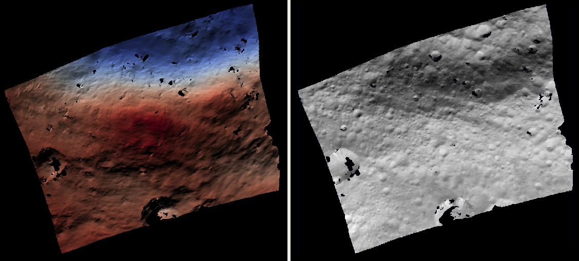
Fig. 8.9 The produced colorized DEM and orthoimage for the CSM Frame camera example. Likely using mapprojection (Section 6.1.7) may have reduced the number and size of the holes in the DEM.

8.12.2. The USGS CSM linescan sensor

In this example we will use the Mars CTX linescan sensor. The images are regular .cub files as in the tutorial in Section 4.2, hence the only distinction compared to that example is that the cameras are stored as .json files.

We will work with the dataset pair:

J03_045994_1986_XN_18N282W.cub J03_046060_1986_XN_18N282W.cub

which, for simplicity, we will rename to left.cub and right.cub and the same for the associated camera files.

See Section 8.14 for another linescan example for the Kaguya linescan sensor for the Moon.

8.12.2.1. Creation CSM linescan cameras

Note that this recipe looks a little different for Frame and SAR cameras, as can be seen in Section 8.12.1.2 and Section 8.12.4.2.

Run the ISIS spiceinit command on the .cub files as:

spiceinit from = left.cub  shape = ellipsoid
spiceinit from = right.cub shape = ellipsoid

Create a conda environment for the ale package:

conda create -c conda-forge -n ale_env python=3.6 ale
conda activate ale_env

(other versions of Python may result in a runtime error later).

Create a Python script named gen_csm_linescan.py:

#!/usr/bin/python

import ale, os, sys

# Get the input cub
cub_file = sys.argv[1]

# Form the output cub
isd_file = os.path.splitext(cub_file)[0] + '.json'

print("Reading: " + cub_file)
usgscsm_str = ale.loads(cub_file)

print("Writing: " + isd_file)
with open(isd_file, 'w') as isd_file:
    isd_file.write(usgscsm_str)

Assuming that conda installed this environment in the default location, run:

$HOME/miniconda3/envs/ale_env/bin/python gen_csm_linescan.py camera.cub

This will produce left.json and right.json.

8.12.2.2. Running stereo

parallel_stereo --stereo-algorithm asp_mgm         \
  --subpixel-mode 9                                \
   left.cub right.cub left.json right.json run/run
point2dem -r mars --stereographic --proj-lon 77.4  \
   --proj-lat 18.4 run/run-PC.tif

Check the stereo convergence angle as printed during preprocessing (Section 8.1). If that angle is small, the results are not going to be great.

See Section 6 for a discussion about various stereo algorithms and speed-vs-quality choices.

The actual stereo session used is csm, and here it will be auto-detected based on the extension of the camera files. For point2dem we chose to use a stereographic projection centered at some point in the area of interest. The fancier MGM algorithm could be used by running this example with --stereo-algorithm asp_mgm.

One can also run parallel_stereo with mapprojected images (Section 6.1.7). The first step would be to create a low-resolution smooth DEM from the previous cloud:

point2dem  -r mars --stereographic --proj-lon 77.4 \
  --proj-lat 18.4 run/run-PC.tif --tr 120          \
  -o run/run-smooth

followed by mapprojecting onto it and redoing stereo:

mapproject --tr 6 run/run-smooth-DEM.tif left.cub  \
  left.json left.map.tif
mapproject --tr 6 run/run-smooth-DEM.tif right.cub \
 right.json right.map.tif
parallel_stereo --stereo-algorithm asp_mgm         \
  --subpixel-mode 9                                \
  left.map.tif right.map.tif left.json right.json  \
  run_map/run run/run-smooth-DEM.tif

Notice how we used the same resolution for both images when mapprojecting. That helps making the resulting images more similar and reduces the processing time (Section 6.1.7.4).

8.12.3. CSM Pushframe sensor

The USGS CSM Pushframe sensor models a pushframe camera. The support for this sensor is not fully mature, and some artifacts can be seen in the DEMs (per below).

What follows is an illustration of using this sensor with Lunar Reconnaissance Orbiter (LRO) WAC images.

This example, including the inputs, recipe, and produced terrain model can be downloaded.

8.12.3.1. Fetching the data

We will focus on the monochromatic images for this sensor. Visit:

https://ode.rsl.wustl.edu/moon/indexproductsearch.aspx

Find the Lunar Reconnaissance Orbiter -> Experiment Data Record Wide Angle Camera - Mono (EDRWAM) option.

Search either based on a longitude-latitude window, or near a notable feature, such as a named crater. We choose a couple of images having the Tycho crater, with download links:

http://pds.lroc.asu.edu/data/LRO-L-LROC-2-EDR-V1.0/LROLRC_0002/DATA/MAP/2010035/WAC/M119923055ME.IMG
http://pds.lroc.asu.edu/data/LRO-L-LROC-2-EDR-V1.0/LROLRC_0002/DATA/MAP/2010035/WAC/M119929852ME.IMG

Fetch these with wget.

8.12.3.2. Creation of .cub files

We broadly follow the tutorial at [Ohman15]. For a dataset called image.IMG, do:

lrowac2isis from = image.IMG to = image.cub

This will create so-called even and odd datasets, with names like image.vis.even.cub and image.vis.odd.cub.

Run spiceinit on them to set up the SPICE kernels:

spiceinit from = image.vis.even.cub
spiceinit from = image.vis.odd.cub

followed by lrowaccal to adjust the image intensity:

lrowaccal from = image.vis.even.cub to = image.vis.even.cal.cub
lrowaccal from = image.vis.odd.cub  to = image.vis.odd.cal.cub

All these .cub files can be visualized with stereo_gui. It can be seen that instead of a single contiguous image we have a set of narrow horizontal framelets, with some of these in the even and some in the odd cub file. The framelets may also be recorded in reverse.

8.12.3.3. Production of seamless mapprojected images

This is not needed for stereo, but may be useful for readers who would like to produce image mosaics using cam2map.

cam2map from = image.vis.even.cal.cub to = image.vis.even.cal.map.cub
cam2map from = image.vis.odd.cal.cub  to = image.vis.odd.cal.map.cub  \
  map = image.vis.even.cal.map.cub matchmap = true

Note how in the second cam2map call we used the map and matchmap arguments. This is to ensure that both of these output images have the same resolution and projection. In particular, if more datasets are present, it is suggested for all of them to use the same previously created .cub file as a map reference. That because stereo works a lot better on mapprojected images with the same ground resolution. For more details see Section 6.1.7 and Section 11.4.2.

To verify that the obtained images have the same ground resolution, do:

gdalinfo image.vis.even.cal.map.cub | grep -i "pixel size"
gdalinfo image.vis.odd.cal.map.cub  | grep -i "pixel size"

(see Section 16.24 regarding this tool).

The fusion happens as:

ls image.vis.even.cal.map.cub image.vis.odd.cal.map.cub  > image.txt
noseam fromlist = image.txt to = image.noseam.cub SAMPLES=73 LINES=73

The obtained file image.noseam.cub may still have some small artifacts but should be overall reasonably good.

8.12.3.4. Stitching the raw even and odd images

This requires ISIS newer than version 6.0, or the latest development code.

For each image in the stereo pair, stitch the even and odd datasets:

framestitch even = image.vis.even.cal.cub odd = image.vis.odd.cal.cub \
  to = image.cub flip = true num_lines_overlap = 2

The flip flag is needed if the order of framelets is reversed relative to what the image is expected to show.

The parameter num_lines_overlap is used to remove a total of this many lines from each framelet (half at the top and half at the bottom) before stitching, in order to deal with the fact that the even and odd framelets have a little overlap, and that they also tend to have artifacts due to some pixels flagged as invalid in each first and last framelet row.

The CSM camera models will assume that this parameter is set at 2, so it should not be modified. Note however that WAC framelets may overlap by a little more than that, so resulting DEMs may have some artifacts at framelet borders, as can be seen further down.

8.12.3.5. Creation of CSM WAC cameras

CSM is a standard for describing camera models (Section 8.12).

The support in ISIS and ASP for pushframe sensors in CSM format is a work in progress. For the time being one should fetch the latest ALE and its conda environment from GitHub, at:

https://github.com/USGS-Astrogeology/ale

then create a script named gen_csm_wac.py:

#!/usr/bin/python

import os, sys
import json
import ale

prefix = sys.argv[1]

if prefix.endswith(".cub") or prefix.lower().endswith(".img") \
  or prefix.endswith(".lbl"):
  prefix = os.path.splitext(prefix)[0]

cub_file = prefix + '.cub'

print("Loading cub file: " + cub_file)

kernels = ale.util.generate_kernels_from_cube(cub_file, expand = True)

usgscsm_str = ale.loads(cub_file, formatter = "ale", \
                    props={"kernels": kernels},
                    verbose = True)

csm_isd = prefix + '.json'
print("Saving: " + csm_isd)
with open(csm_isd, 'w') as isd_file:
  isd_file.write(usgscsm_str)

Invoke it with either the even or odd .cub file as an argument. For example:

$HOME/miniconda3/envs/ale_env/bin/python gen_csm_wac.py \
  image.vis.even.cal.cub

Do not use the stitched .cub file as that one lacks camera information. The obtained .json files can be renamed to follow the same convention as the stitched .cub images.

At some point when a new version of ISIS is released (version > 6), it may have a tool for creation of CSM camera models.

8.12.3.6. Running stereo

parallel_stereo --stereo-algorithm asp_mgm   \
  --left-image-crop-win 341 179 727 781      \
  --right-image-crop-win 320 383 824 850     \
  M119923055ME.cub M119929852ME.cub          \
  M119923055ME.json M119929852ME.json        \
  run/run

point2dem run/run-PC.tif --orthoimage run/run-L.tif
hillshade run/run-DEM.tif
colormap run/run-DEM.tif -s run/run-DEM_HILLSHADE.tif

As printed by stereo_pprc, the convergence angle is about 27 degrees, which is a good number.

See Section 6 for a discussion about various stereo speed-vs-quality choices.

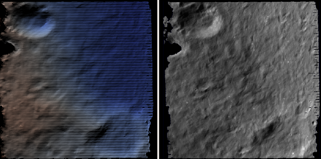
Fig. 8.10 The produced colorized DEM and orthoimage for the CSM WAC camera example. The artifacts are due to issues stitching of even and odd framelets.

It can be seen that the stereo DEM has some linear artifacts. That is due to the fact that the stitching does not perfectly integrate the framelets.

An improved solution can be obtained by creating a low-resolution version of the above DEM, mapprojecting the images on it, and then re-running stereo, per (Section 6.1.7).

point2dem --tr 0.03 run/run-PC.tif --search-radius-factor 5 -o \
  run/run-low-res
mapproject --tr 0.0025638 run/run-low-res-DEM.tif              \
  M119923055ME.cub M119923055ME.json M119923055ME.map.tif
mapproject --tr 0.0025638 run/run-low-res-DEM.tif              \
  M119929852ME.cub M119929852ME.json M119929852ME.map.tif
parallel_stereo --stereo-algorithm asp_mgm                     \
  M119923055ME.map.tif M119929852ME.map.tif                    \
  M119923055ME.json M119929852ME.json                          \
  run_map/run run/run-low-res-DEM.tif
point2dem run_map/run-PC.tif --orthoimage run_map/run-L.tif
hillshade run_map/run-DEM.tif
colormap run_map/run-DEM.tif -s run_map/run-DEM_HILLSHADE.tif

To create the low-resolution DEM we used a grid size which is about 10 times coarser than the one for the DEM created earlier. Note that the same resolution is used when mapprojecting both images; that is very important to avoid a large search range in stereo later. This is discussed in more detail in Section 6.1.7.

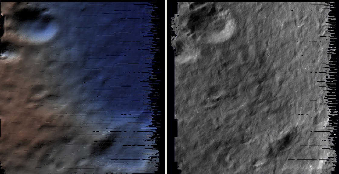
Fig. 8.11 The produced colorized DEM and orthoimage for the CSM WAC camera example, when mapprojected images are used.

As can be seen in the second figure, there are somewhat fewer artifacts. The missing lines in the DEM could be filled in if point2dem was run with --search-radius-factor 4, for example.

Given that there exists a wealth of WAC images, one could also try to get several more stereo pairs with similar illumination, run bundle adjustment for all of them (Section 16.5), run pairwise stereo, create DEMs (at the same resolution), and then merge them with dem_mosaic (Section 16.19). This may further attenuate the artifacts as each stereo pair will have them at different locations. See Section 8.1 for guidelines about how to choose good stereo pairs.

8.12.4. The USGS CSM SAR sensor for LRO Mini-RF

Mini-RF was a Synthetic Aperture Radar (SAR) sensor on the LRO spacecraft. It is challenging to process its data with ASP for several reasons:

• The synthetic image formation model produces curved rays going from the ground to the pixel in the camera ([KBW+16]). To simplify the calculations, ASP finds where a ray emanating from the camera intersects the standard Moon ellipsoid with radius 1737.4 km and declares the ray to be a straight line from the camera center to this point.

• This sensor very rarely acquires stereo pairs. The convergence angle (Section 8.1) as printed by parallel_stereo in pre-processing is usually less than 5 degrees, which is little and results in noisy DEMs. In this example we will use a dataset intentionally created with stereo in mind. The images will cover a part of Jackson crater ([KHKB+11]).

• It is not clear if all modeling issues with this sensor were resolved. The above publication states that “Comparison of the stereo DTM with ~250 m/post LOLA grid data revealed (in addition to dramatically greater detail) a very smooth discrepancy that varied almost quadratically with latitude and had a peak-to-peak amplitude of nearly 4000 m.”

• The images are dark and have unusual appearance, which requires some pre-processing and a large amount of interest points.

Hence, ASP’s support for this sensor is experimental. The results are plausible but likely not fully rigorous.

This example, including input images, produced outputs, and a recipe, is available for download at:

https://github.com/NeoGeographyToolkit/StereoPipelineSolvedExamples

No ISIS data are needed to run it.

8.12.4.1. Creating the input images

Fetch the data from PDS:

wget https://pds-geosciences.wustl.edu/lro/lro-l-mrflro-4-cdr-v1/lromrf_0002/data/sar/03800_03899/level1/lsz_03821_1cd_xku_16n196_v1.img
wget https://pds-geosciences.wustl.edu/lro/lro-l-mrflro-4-cdr-v1/lromrf_0002/data/sar/03800_03899/level1/lsz_03821_1cd_xku_16n196_v1.lbl
wget https://pds-geosciences.wustl.edu/lro/lro-l-mrflro-4-cdr-v1/lromrf_0002/data/sar/03800_03899/level1/lsz_03822_1cd_xku_23n196_v1.img
wget https://pds-geosciences.wustl.edu/lro/lro-l-mrflro-4-cdr-v1/lromrf_0002/data/sar/03800_03899/level1/lsz_03822_1cd_xku_23n196_v1.lbl

These will be renamed to left.img, right.img, etc., to simply the processing.

Create .cub files:

export ISISROOT=$HOME/miniconda3/envs/isis6
export PATH=$ISISROOT/bin:$PATH
export ISISDATA=$HOME/isis3data

mrf2isis from = left.lbl  to = left.cub
mrf2isis from = right.lbl to = right.cub

Run spiceinit. Setting the shape to the ellipsoid makes it easier to do image-to-ground computations and is strongly suggested:

spiceinit from = left.cub  shape = ellipsoid
spiceinit from = right.cub shape = ellipsoid

8.12.4.2. Creation of CSM SAR cameras

Fetch the latest ale from GitHub:

https://github.com/USGS-Astrogeology/ale

or something newer than version 0.8.7 on conda-forge, which lacks certain functionality for SAR. Below we assume a very recent version of USGS CSM, as shipped with ASP. Version 1.5.2 of this package on conda-forge is too old for the following to work.

Create a script called gen_csm_sar.py. (Note that this script differs somewhat for analogous scripts earlier in the text, at Section 8.12.1.2 and Section 8.12.2.1.)

#!/usr/bin/python

import os, sys
import json
import ale

prefix = sys.argv[1]

if prefix.lower().endswith(".cub") or prefix.lower().endswith(".img") \
  or prefix.lower().endswith(".lbl"):
  # Remove extension
  prefix = os.path.splitext(prefix)[0]

cub_file = prefix + '.cub'
print("Loading cub file: " + cub_file)

kernels = ale.util.generate_kernels_from_cube(cub_file, expand = True)
usgscsm_str = ale.loads(cub_file, formatter = "ale", \
  props={"kernels": kernels}, verbose = False)

csm_isd = prefix + '.json'
print("Saving: " + csm_isd)
with open(csm_isd, 'w') as isd_file:
  isd_file.write(usgscsm_str)

Run it as:

$HOME/miniconda3/envs/ale_env/bin/python gen_csm_sar.py left.cub
$HOME/miniconda3/envs/ale_env/bin/python gen_csm_sar.py right.cub

The above paths will need adjusting for your system. The path to Python should be such that the recently installed ale is picked up.

Run cam_test (Section 16.9) as a sanity check:

cam_test --image left.cub  --cam1 left.cub  --cam2 left.json
cam_test --image right.cub --cam1 right.cub --cam2 right.json

8.12.4.3. Preparing the images

ASP accepts only single-band images, while these .cub files have four of them. We will pull the first band and clamp it to make it easier for stereo to find interest point matches:

gdal_translate -b 1 left.cub  left_b1.tif
gdal_translate -b 1 right.cub right_b1.tif

image_calc -c "min(var_0, 0.5)" left_b1.tif  -d float32 \
  -o left_b1_clamp.tif
image_calc -c "min(var_0, 0.5)" right_b1.tif -d float32 \
  -o right_b1_clamp.tif

8.12.4.4. Running stereo

It is simpler to first run a clip with stereo_gui (Section 16.67). This will result in the following command:

parallel_stereo --ip-per-tile 3500             \
  --left-image-crop-win 0 3531 3716 10699      \
  --right-image-crop-win -513 22764 3350 10783 \
  --stereo-algorithm asp_mgm --min-num-ip 10   \
  left_b1_clamp.tif right_b1_clamp.tif         \
  left.json right.json run/run

The stereo convergence angle for this pair is 18.4 degrees which is rather decent.

Create a colorized DEM and orthoimage:

point2dem run/run-PC.tif --orthoimage run/run-L.tif
hillshade run/run-DEM.tif
colormap run/run-DEM.tif -s run/run-DEM_HILLSHADE.tif

See Section 6 for a discussion about various speed-vs-quality choices when running stereo.

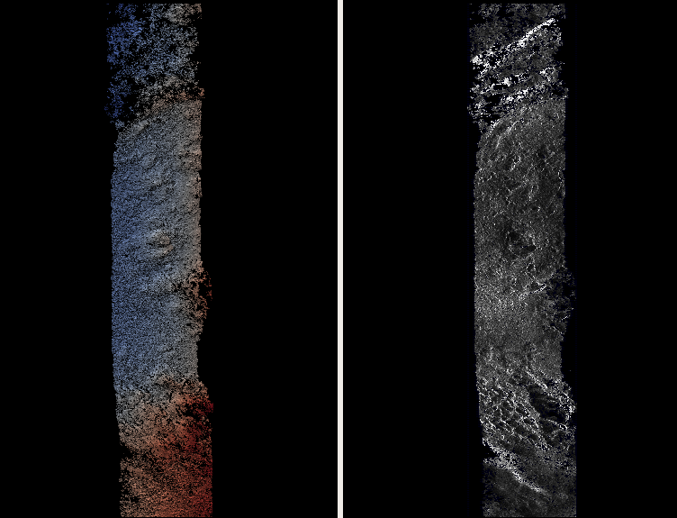
Fig. 8.12 The produced colorized DEM and orthoimage for the CSM SAR example.

8.12.5. CSM cameras for MSL

This example shows how, given a set of Mars Science Laboratory (MSL) Curiosity rover Nav or Mast camera images, CSM camera models can be created. Stereo pairs are then used (with either Nav or Mast data) to make DEMs and orthoimages.

After recent fixes in ALE (details below), the camera models are accurate enough that stereo pairs acquired at different rover locations and across different days result in consistent DEMs and orthoimages.

See Section 9.3 for a Structure-from-Motion solution without using CSM cameras. That one results in self-consistent meshes that, unlike the DEMs produced here, are not geolocated.

8.12.5.1. Illustration

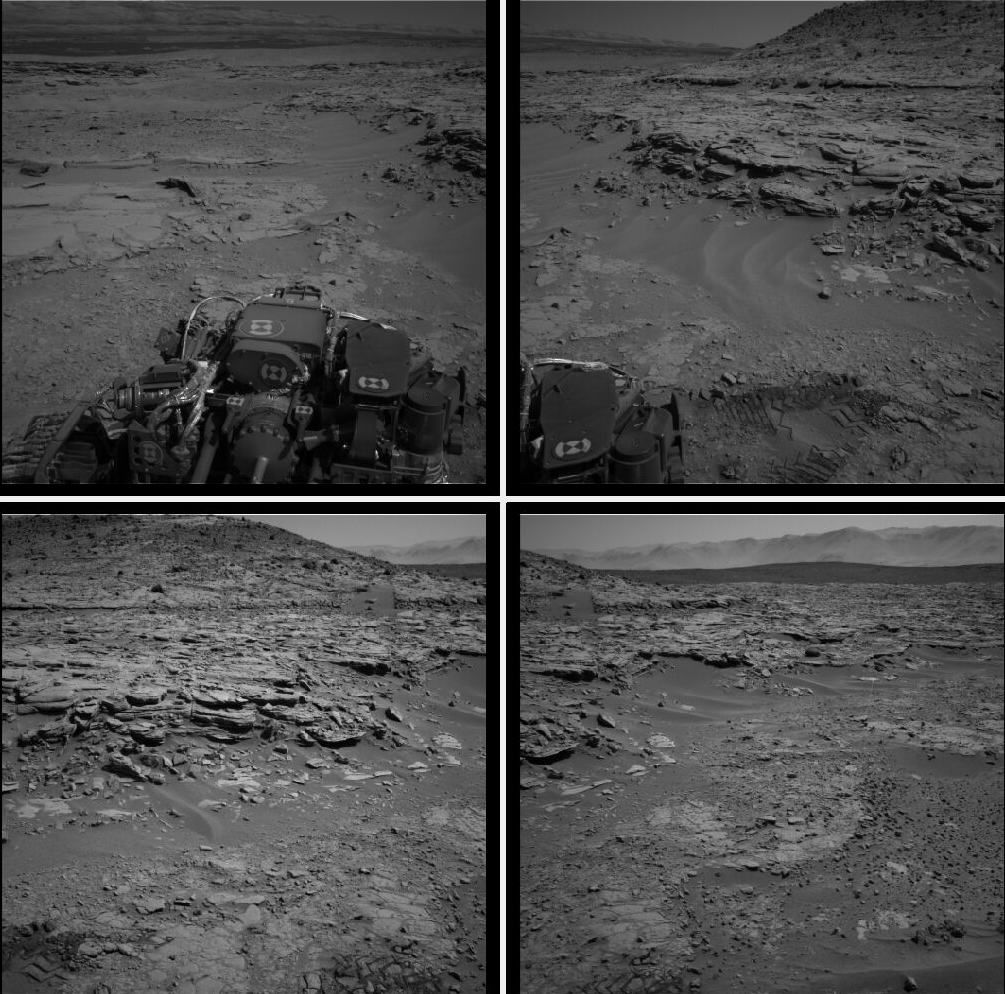
Fig. 8.13 Four out of the 10 images (5 stereo pairs) used in this example.

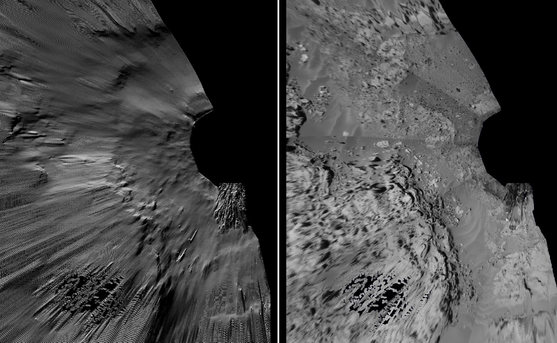
Fig. 8.14 Produced DEM and orthoimage. See Section 8.12.5.7 for a larger example.

8.12.5.2. Fetch the images and metadata from PDS

See Section 9.3.4. Here we will work with .cub files rather than converting them to .png. The same Mars day will be used as there (SOL 597). The datasets for SOL 603 were verified to work as well.

The dataset used in this example (having .LBL, .cub, and .json files) is available for download. It is suggested to recreate the .json files in that dataset in view of the recent updates to ALE.

8.12.5.3. Download the SPICE data

The .LBL metadata files from PDS do not have the SPICE data that is needed to find the position and orientation of the MSL rover on Mars. For that, need to fetch the SPICE kernels from the USGS ISIS server.

Get a recent version of rclone.conf for ISIS:

wget https://raw.githubusercontent.com/USGS-Astrogeology/ISIS3/dev/isis/config/rclone.conf \
-O rclone.conf

Set the ISIS data environmental variable and download the kernels (adjust the path below):

export ISISDATA=/path/to/isisdata
mkdir -p $ISISDATA
downloadIsisData msl $ISISDATA --config rclone.conf

The downloadIsisData script is shipped with ISIS (Section 2.1.3).

8.12.5.4. Set up ALE

The functionality for creating CSM camera models is available in the ALE package. For the time being, handling the MSL cameras requires fetching the latest code from GitHub:

git clone git@github.com:DOI-USGS/ale.git

Also create a supporting conda environment:

cd ale
conda env create -n ale -f environment.yml

See Section 2.3 for how to install conda.

Make sure Python can find the needed routines (adjust the path below):

export PYTHONPATH=/path/to/ale

8.12.5.5. Creation of CSM MSL cameras

ALE expects the following variable to be set:

export ALESPICEROOT=$ISISDATA

A full-resolution MSL left Nav image uses the naming convention:

NLB_<string>_F<string>.cub

with the right image starting instead with NRB. The metadata files downloaded from PDS end with .LBL.

Create a Python script called gen_csm_msl.py with the following code:

#!/usr/bin/python

import os, sys, json, ale

labelFile = sys.argv[1]
prefix = os.path.splitext(labelFile)[0]
usgscsm_str = ale.loads(labelFile, formatter = "ale",
                        verbose = True)

csm_isd = prefix + '.json'
print("Saving: " + csm_isd)
with open(csm_isd, 'w') as isd_file:
  isd_file.write(usgscsm_str)

A CSM camera file can be created by running this script as:

$HOME/miniconda3/envs/ale_env/bin/python gen_csm_msl.py image.LBL

This will produce the file image.json. We called the Python program from the newly created conda environment.

One may get an error saying:

The first file
'/usgs/cpkgs/isis3/data/msl/kernels/lsk/naif0012.tls'
specified by KERNELS_TO_LOAD in the file
/path/to/isisdata/msl/kernels/mk/msl_v01.tm
could not be located.

That is due to a bug in the ISIS data. Edit that .tls file and specify the correct location of msl_v01.tm in your ISIS data directory. Once things are working, the verbose flag can be set to False in the above script.

8.12.5.6. Simple stereo example

In this example the camera orientations are not refined using bundle adjustment, as the camera poses are reasonably good. If desired to do that, one could run bundle_adjust (Section 16.5) as:

bundle_adjust --no-datum --camera-weight 0 --tri-weight 0.1 \
  data/*.cub data/*.json -o ba/run

Here and below we use the option --no-datum as these are ground-level cameras, when rays emanating from them may not reliably intersect the planet datum.

For each stereo pair, run parallel_stereo (Section 16.50) as:

parallel_stereo                 \
  --stereo-algorithm asp_mgm    \
  --subpixel-mode 3 --no-datum  \
  --min-triangulation-angle 1.5 \
  left.cub right.cub            \
  left.json right.json          \
  run/run

If bundle adjustment was used, the above command should be run with the option --bundle-adjust-prefix ba/run.

The option --min-triangulation-angle 1.5 is highly essential. It filters out far-away and noisy points. Increasing this will remove more points. For terrains with a lot of shadows (such as for the Moon), also consider using the option --no-data-value to filter out pixels with low intensity (Section 17).

This is followed by DEM and orthoimage creation (Section 16.55) with:

point2dem --stereographic                \
  --proj-lon 137.402 --proj-lat -4.638   \
  --search-radius-factor 5 --orthoimage  \
  run/run-PC.tif run/run-L.tif

Here, the option --search-radius-factor 5 is used to fill the point cloud when moving further from the rover. A local stereographic projection was used.

The produced DEMs can be mosaicked together with dem_mosaic (Section 16.19) as:

dem_mosaic */*DEM.tif -o dem_mosaic.tif

For the orthoimages, one can use:

dem_mosaic --first */*DRG.tif -o ortho_mosaic.tif

The option --first picks the first encountered image pixel at each location, rather than blending them together which may blur the output mosaic.

See an illustration in Fig. 8.14, with the input images in Fig. 8.13.

8.12.5.7. Multi-day stereo

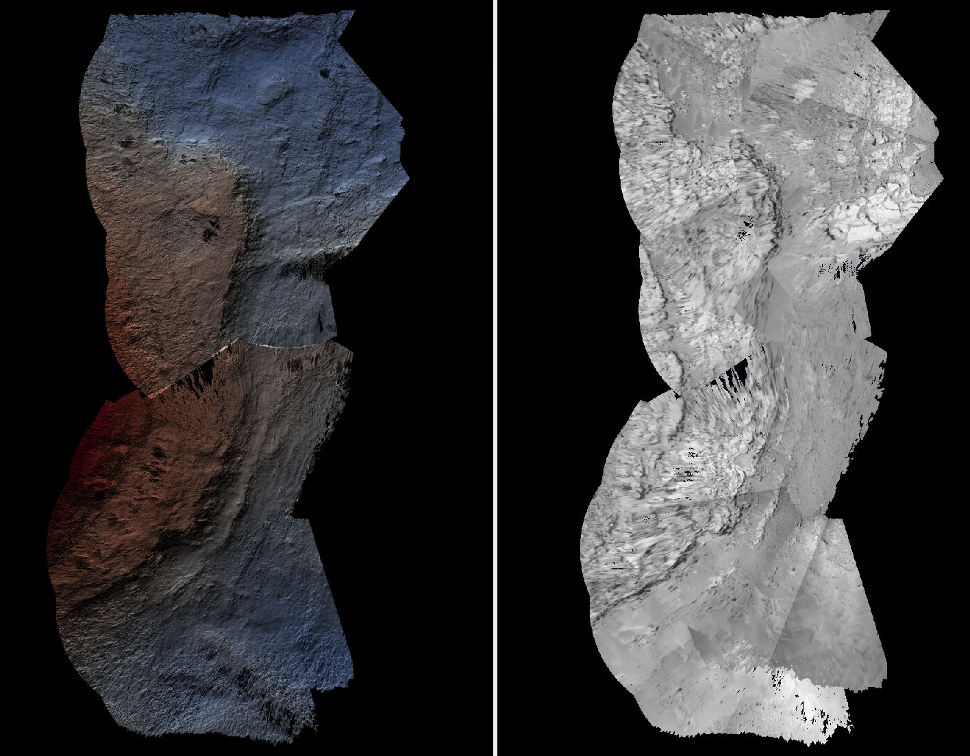
Fig. 8.15 A combined DEM and orthoimage produced from 15 stereo pairs from SOL 597 and 13 stereo pairs from SOL 603. The misregistration half-way down is not due to mismatch across days but because of insufficient overlap between two image subsets on SOL 603. Here, blue and red correspond to elevations of -5038.921 and -5034.866 meters.

In this example we take advantage of the fact that there is decent overlap between images acquired on SOL 597 and SOL 603. They both image the same hill, called Kimberly, in Gale crater, from somewhat different perspectives. Hence we combine these datasets to increase the coverage.

Good overlap between different days, or even between consecutive rover stops in the same day, is not guaranteed. Sometimes the low-resolution nav cam images (Section 8.12.5.10) can help with increasing the overlap and coverage. Lack of good overlap can result in registration errors, as can be seen in Fig. 8.15.

For a larger and better-behaved dataset it is suggested to consider the images from SOL 3551 to 3560. Some effort may be needed to select a good subset.

A workflow can be follows. First, individual DEMs were created and mosaicked, as in Section 8.12.5. The quality of the produced DEM can be quite uneven, especially far from the camera.

Large holes in the initial DEM were filled in with the dem_mosaic option --fill-search-radius (Section 16.19.2.8).

Then, it can be made coarser, for example, as:

gdalwarp -r cubic -tr 0.1 0.1 input.tif output.tif

(This assumes the projection is local stereographic.)

This DEM was then blurred a few times with dem_mosaic option --dem-blur-sigma 10. This should be repeated until the DEM is smooth enough and shows no artifacts. The resulting DEM is called dem.tif.

All images were mapprojected onto this DEM using the same local stereographic projection, and a resolution of 0.01 m:

proj="+proj=stere +lat_0=-4.638 +lon_0=137.402 +k=1 +x_0=0 +y_0=0 +R=3396190 +units=m +no_defs"
mapproject --tr 0.01 --t_srs "$proj" \
  dem.tif image.cub image.json image.map.tif

Bundle adjustment was run on the desired set of input images and cameras, while making use of the mapprojected images to find matches:

dem=dem.tif
parallel_bundle_adjust                    \
  --image-list images.txt                 \
  --camera-list cameras.txt               \
  --mapprojected-data-list map_images.txt \
  --camera-weight 0                       \
  --heights-from-dem $dem                 \
  --heights-from-dem-uncertainty 10.0     \
  --heights-from-dem-robust-threshold 0.1 \
  --auto-overlap-params "$dem 15"         \
  -o ba/run

In retrospect, this mapprojection step may be not necessary, and one could run bundle adjustment with original images.

Then parallel_stereo was run with mapprojected images, with the option --bundle-adjust-prefix ba/run, to use the bundle-adjusted cameras:

parallel_stereo                    \
  --stereo-algorithm asp_mgm       \
  --subpixel-mode 9                \
  --max-disp-spread 80             \
  --min-triangulation-angle 1.5    \
  --bundle-adjust-prefix ba/run    \
  left.map.tif right.map.tif       \
  left.json right.json run_map/run \
  $dem

point2dem --tr 0.01 --stereographic    \
  --proj-lon 137.402 --proj-lat -4.638 \
  --errorimage                         \
  run_map/run-PC.tif                   \
  --orthoimage run_map/run-L.tif

Each run must use a separate output prefix, instead of run_map/run.

Here, the option --min-triangulation-angle 1.5 was highly essential. It filters out far-away and noisy points.

Even with this option, the accuracy of a DEM goes down far from the cameras. Artifacts can arise where the same region is seen from two different locations, and it is far from either. In this particular example some problematic portions were cut out with gdal_rasterize (Section 16.67.7.2).

The produced DEMs were inspected, and the best ones were mosaicked together with dem_mosaic, as follows:

dem_mosaic --weights-exponent 0.5 */*DEM.tif -o dem_mosaic.tif

The option --weights-exponent 0.5 reduced the artifacts in blending.

The orthoimages were mosaicked with:

dem_mosaic --first */*DRG.tif -o ortho_mosaic.tif

It is suggested to sort the input images for this call from best to worst in terms of quality. In particular, the images where the rover looks down rather towards the horizon should be earlier in the list.

See the produced DEM and orthoimage in Fig. 8.15.

8.12.5.8. Mapprojection

The input .cub image files and the camera .json files can be used to create mapprojected images with the mapproject program (Section 16.40). The DEM for mapprojection can be the one created earlier with point2dem. If a third-party DEM is used, one has to make sure its elevations are consistent with the DEMs produced earlier.

Use the option --t_projwin to prevent the produced images from extending for a very long distance towards the horizon.

8.12.5.9. MSL Mast cameras

The same procedure works for creating MSL Mast cameras. To run stereo, first use gdal_translate -b 1 to pull the first band from the input images. This workflow was tested with the stereo pair 0706ML0029980010304577C00_DRCL and 0706MR0029980000402464C00_DRCL for SOL 706.

8.12.5.10. Low-resolution MSL Nav cam images

In addition to full-resolution Nav camera images (1024 pixels), MSL also acquires low-resolution Nav images (256 pixels) at separate times. These have the string _D as part of their name, instead of _F. Such images were validated to work, and can produce good DEMs that can plug some gaps in coverage.

8.12.6. CSM model state

CSM cameras are stored in JSON files, in one of the following two formats:

• ISD: It has the transforms from sensor coordinates to J2000, and from J2000 to ECEF.

• Model state: Then the above-mentioned transforms are combined, and other information is condensed or removed.

The model state files have all the data needed to project ground points into the camera and vice-versa, so they are sufficient for any use in ASP. The model state can also be embedded in ISIS cubes (Section 8.12.7).

ASP’s bundle adjustment program (Section 16.5) normally writes plain text .adjust files which encode how the position and orientation of the cameras were modified (Section 16.5.12). If invoked for CSM cameras, additional files with extension .adjusted_state.json are saved in the same output directory, which contain the model state from the input CSM cameras with the optimization adjustments applied to them (use zero iterations in bundle_adjust to save the states of the original cameras).

This functionality is implemented for all USGS CSM sensors, so, for frame, linescan, pushframe, and SAR models.

The cam_gen program can convert several linescan camera model types to CSM model state (Section 16.8.1.5). It can also approximate some Pinhole, RPC, or other cameras with CSM frame cameras in model state format (Section 16.8.1.4). The usgscsm_cam_test program can convert any CSM camera to model state.

ASP’s parallel_stereo and bundle adjustment programs can, in addition to CSM ISD camera model files, also load such model state files, either as previously written by ASP or from an external source (it will auto-detect the type from the format of the JSON files). Hence, the model state is a convenient format for data exchange, while being less complex than the ISD format.

If parallel_stereo is used to create a point cloud from images and CSM cameras, and then that point cloud has a transform applied to it, such as with pc_align, the same transform can be applied to the model states for the cameras using bundle_adjust (Section 16.52.14).

To evaluate how well the obtained CSM camera approximates the ISIS camera model, run the program cam_test shipped with ASP (Section 16.9) as follows:

cam_test --sample-rate 100 --image camera.cub \
  --cam1 camera.cub --cam2 camera.json

The pixel errors are expected to be at most on the order of 0.2 pixels.

8.12.7. CSM state embedded in ISIS cubes

ASP usually expects CSM cameras to be specified in JSON files. It also accepts CSM camera model state data (Section 8.12.6) embedded in ISIS cubes, if all of the following (reasonable) assumptions are satisfied:

• JSON files are not passed in.

• The ISIS cubes contain CSM model state data (in the CSMState group).

• The --session-type (or --t) option value is not set to isis (or isismapisis). So, its value should be either csm (or csmmapcsm), or left blank.

Hence, if no CSM data is provided, either in the ISIS cubes or separately in JSON files, or --session-type is set to isis (or isismapisis), ASP will use the ISIS camera models.

The above applies to all ASP tools that read CSM cameras (parallel_stereo, bundle_adjust, jitter_solve, mapproject, cam_test).

If bundle_adjust (Section 16.5) or jitter_solve (Section 16.37) is run with CSM cameras, either embedded in ISIS cubes or specified separately, and the flag --update-isis-cubes-with-csm-state is set, then the optimized model states will be saved back to the ISIS cubes, while the SPICE and other obsolete information from the cubes will be deleted (spiceinit can be used to restore the cubes). Separate model state files in the JSON format will be saved as well, as done without this option.

Note that if images are mapprojected with certain camera files, and then those camera files are updated in-place, this will result in wrong results if stereo is run with the mapprojected images and updated cameras.

See also the csminit and spiceinit documentation.