11. Technical discussion

In this chapter we will dive much deeper into understanding the core algorithms in the Stereo Pipeline. We start with an overview of the five stages of stereo reconstruction. Then we move into an in-depth discussion and exposition of the various correlation algorithms.

The goal of this chapter is to build an intuition for the stereo correlation process. This will help users to identify unusual results in their DEMs and hopefully eliminate them by tuning various parameters in the stereo.default file (Section 17). For scientists and engineers who are using DEMs produced with the Stereo Pipeline, this chapter may help to answer the question, “What is the Stereo Pipeline doing to the raw data to produce this DEM?”

A related question that is commonly asked is, “How accurate is a DEM produced by the Stereo Pipeline?” This chapter does not yet address matters of accuracy and error, however we have several efforts underway to quantify the accuracy of Stereo Pipeline-derived DEMs, and will be publishing more information about that shortly. Stay tuned.

The entire stereo correlation process, from raw input images to a point cloud or DEM, can be viewed as a multistage pipeline as depicted in Fig. 11.1, and detailed in the following sections.

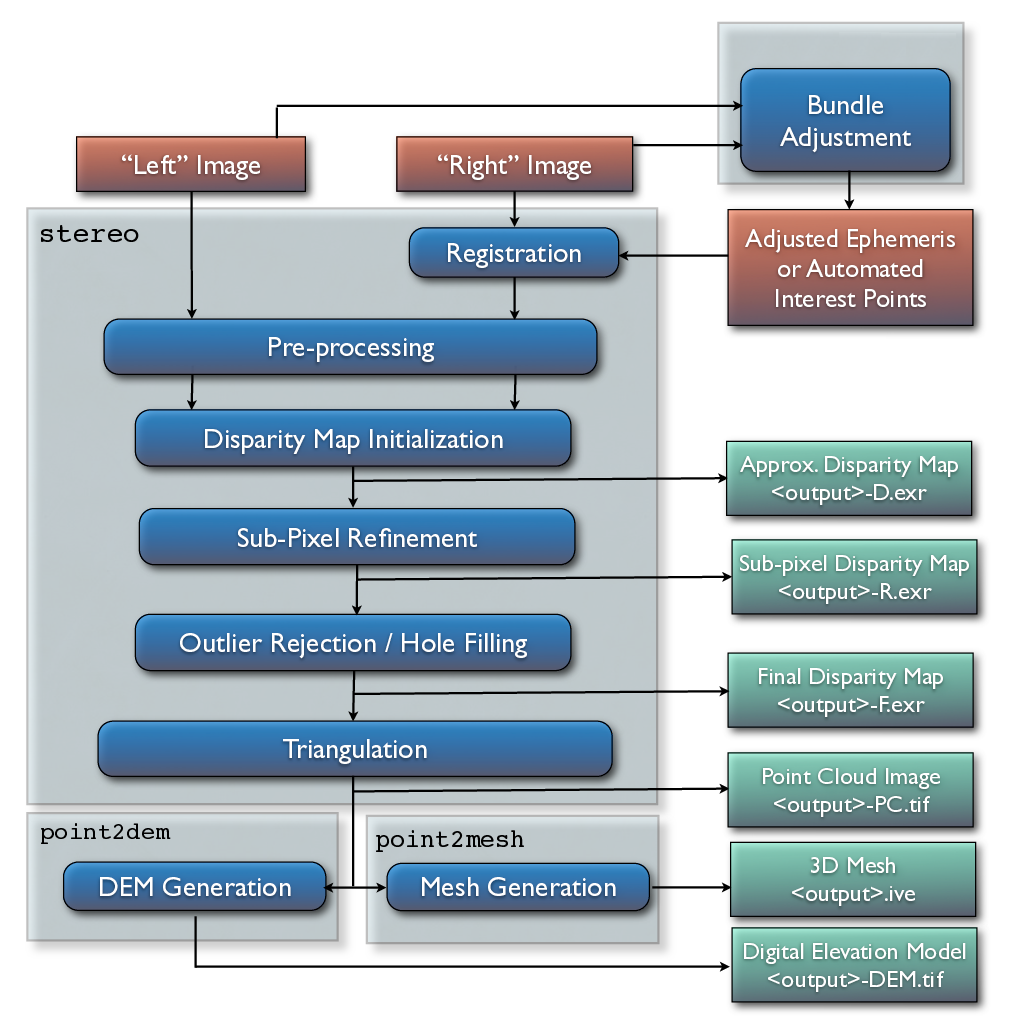
Fig. 11.1 Flow of data through the Stereo Pipeline.

11.1. Pre-processing

The first optional (but recommended) step in the process is least squares Bundle Adjustment, which is described in detail in Section 12.

Next, the left and right images are roughly aligned using one of the four methods: (1) a homography transform of the right image based on automated tie-point measurements, (2) an affine epipolar transform of both the left and right images (also based on tie-point measurements as earlier), the effect of which is equivalent to rotating the original cameras which took the pictures, (3) a 3D rotation that achieves epipolar rectification (only implemented for Pinhole sessions for missions like MER or K10, see Section 8.6 and Section 8.7) or (4) map-projection of both the left and right images using the ISIS cam2map command or through the more general mapproject tool that works for any cameras supported by ASP (see Section 6.1.7 for the latter). The first three options can be applied automatically by the Stereo Pipeline when the alignment-method variable in the stereo.default file is set to affineepipolar, homography, or epipolar, respectively.

The latter option, running cam2map, cam2map4stereo.py, or mapproject must be carried out by the user prior to invoking the parallel_stereo command. Map-projecting the images using ISIS eliminates any unusual distortion in the image due to the unusual camera acquisition modes (e.g. pitching “ROTO” maneuvers during image acquisition for MOC, or highly elliptical orbits and changing line exposure times for the , HRSC). It also eliminates some of the perspective differences in the image pair that are due to large terrain features by taking the existing low-resolution terrain model into account (e.g. the MOLA, LOLA, NED, or ULCN 2005 models).

In essence, map-projecting the images results in a pair of very closely matched images that are as close to ideal as possible given existing information. This leaves only small perspective differences in the images, which are exactly the features that the stereo correlation process is designed to detect.

For this reason, we recommend map-projection for pre-alignment of most stereo pairs. Its only cost is longer triangulation times as more math must be applied to work back through the transforms applied to the images. In either case, the pre-alignment step is essential for performance because it ensures that the disparity search space is bounded to a known area. In both cases, the effects of pre-alignment are taken into account later in the process during triangulation, so you do not need to worry that pre-alignment will compromise the geometric integrity of your DEM.

In some cases the pre-processing step may also normalize the pixel values in the left and right images to bring them into the same dynamic range. Various options in the stereo.default file affect whether or how normalization is carried out, including individually-normalize and force-use-entire-range. Although the defaults work in most cases, the use of these normalization steps can vary from data set to data set, so we recommend you refer to the examples in Section 8 to see if these are necessary in your use case.

Finally, pre-processing can perform some filtering of the input images (as determined by prefilter-mode) to reduce noise and extract edges in the images. When active, these filters apply a kernel with a sigma of prefilter-kernel-width pixels that can improve results for noisy images (prefilter-mode must be chosen carefully in conjunction with cost-mode, see Section 17). The pre-processing modes that extract image edges are useful for stereo pairs that do not have the same lighting conditions, contrast, and absolute brightness [Nis84]. We recommend that you use the defaults for these parameters to start with, and then experiment only if your results are sub-optimal.

11.2. Disparity map initialization

Correlation is the process at the heart of the Stereo Pipeline. It is a collection of algorithms that compute correspondences between pixels in the left image and pixels in the right image. The map of these correspondences is called a disparity map. This is saved in the file named output_prefix-D.tif.

A disparity map is an image whose pixel locations correspond to the pixel \((u,v)\) in the left image, and whose pixel values contain the horizontal and vertical offsets \((d_u, d_v)\) to the matching pixel in the right image, which is \((u+d_u, v+d_v)\).

The correlation process attempts to find a match for every pixel in the left image. The only pixels skipped are those marked invalid in the mask images. For large images (e.g. from HiRISE, , LROC, or WorldView), this is very expensive computationally, so the correlation process is split into two stages. The disparity map initialization step computes approximate correspondences using a pyramid-based search that is highly optimized for speed, but trades resolution for speed. The results of disparity map initialization are integer-valued disparity estimates. The sub-pixel refinement step takes these integer estimates as initial conditions for an iterative optimization and refines them using the algorithm discussed in the next section.

We employ several optimizations to accelerate disparity map initialization: (1) a box filter-like accumulator that reduces duplicate operations during correlation [Sun02]; (2) a coarse-to-fine pyramid based approach where disparities are estimated using low-resolution images, and then successively refined at higher resolutions; and (3) partitioning of the disparity search space into rectangular sub-regions with similar values of disparity determined in the previous lower resolution level of the pyramid [Sun02].

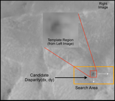
Fig. 11.2 The correlation algorithm in disparity map initialization uses a sliding template window from the left image to find the best match in the right image. The size of the template window can be adjusted using the H_KERN and V_KERN parameters in the stereo.default file, and the search range can be adjusted using the {H,V}_CORR_{MIN/MAX} parameters.

Naive correlation itself is carried out by moving a small, rectangular template window from the from left image over the specified search region of the right image, as in Fig. 11.2. The “best” match is determined by applying a cost function that compares the two windows. The location at which the window evaluates to the lowest cost compared to all the other search locations is reported as the disparity value. The cost-mode variable allows you to choose one of three cost functions, though we recommend normalized cross correlation [Men97], since it is most robust to slight lighting and contrast variations between a pair of images. Try the others if you need more speed at the cost of quality.

11.3. Low-resolution disparity

Producing the disparity map at full resolution as in Section 11.2 is computationally expensive. To speed up the process, ASP starts by first creating a low-resolution initial guess version of the disparity map. This is saved in the file output_prefix-D_sub.tif.

Four methods are available for producing this low-resolution disparity, described below.

11.3.1. Disparity from stereo correlation

The default approach is to use for the low-resolution disparity the same algorithm as for the full-resolution one, but called with the low-resolution images output_prefix-L_sub.tif and output_prefix-R_sub.tif.

Those “sub” images have their size chosen so that their area is around 2.25 megapixels, a size that is easily viewed on the screen unlike the raw source images.

This corresponds to the parallel_stereo option --corr-seed-mode 1 (Section 17).

11.3.2. Disparity from a DEM

The low resolution disparity can be computed from a lower-resolution initial guess DEM of the area. This works with all alignment methods except epipolar (Section 17.1.2). Mapprojected images are supported (Section 6.1.7).

This option assumes rather good alignment between the cameras and the DEM. Otherwise see Section 16.54.14. The option --disparity-estimation-dem-error should be used to specify the uncertainty in such a DEM.

This can be useful when there are a lot of clouds, or terrain features are not seen well at low resolution.

As an example, invoke parallel_stereo with options along the lines of:

--corr-seed-mode 2                 \
--disparity-estimation-dem ref.tif \
--disparity-estimation-dem-error 5

When features are washed out at low resolution, consider also adding the option --corr-max-levels 2, or see Section 11.3.3.

See Section 17 for more information on these options.

It is suggested to extract the produced low-resolution disparity bands with gdal_translate (Section 16.34.1.9) or disparitydebug (Section 16.23). Inspect them in stereo_gui (Section 16.69).

11.3.3. Sparse disparity from full-resolution images

For snowy landscapes, whose only features may be small-scale grooves or ridges sculpted by wind (so-called zastrugi), the low-resolution images appear blank, so the default low-resolution disparity approach in Section 11.3.1 fails.

One can then use a disparity from a DEM (Section 11.3.2), skip the low-resolution disparity (Section 11.3.4), or the approach outlined in this section, based on the tool named sparse_disp.

This program create the low-resolution initial disparity output_prefix-D_sub.tif from the full-resolution images, yet only at a sparse set of pixels for reasons, of speed. This low-resolution disparity is then refined as earlier using a pyramid approach, but with fewer levels, to prevent the features being washed out.

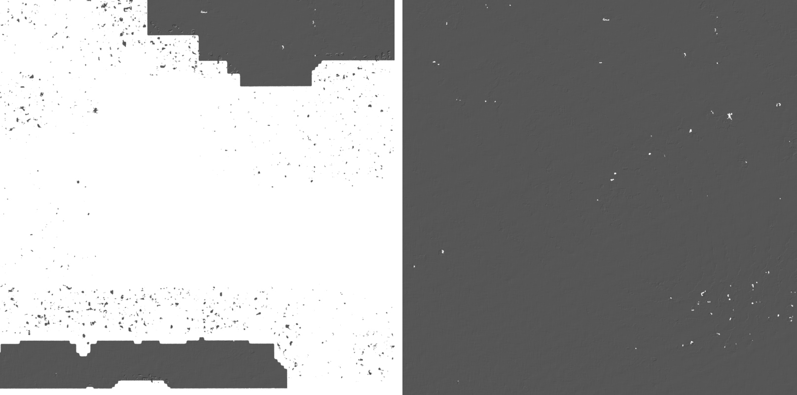
Fig. 11.3 Example of a difficult terrain obtained without (left) and with (right) sparse_disp. (In these DEMs there is very little elevation change, hence the flat appearance.)

Here is an example:

parallel_stereo -t dg --corr-seed-mode 3            \
  --corr-max-levels 2                               \
  left_mapped.tif right_mapped.tif                  \
  12FEB12053305-P1BS_R2C1-052783824050_01_P001.XML  \
  12FEB12053341-P1BS_R2C1-052783824050_01_P001.XML  \
  dg/dg srtm_53_07.tif

This tool can be customized with the parallel_stereo switch --sparse-disp-options.

11.3.3.1. Installation of sparse_disp

The sparse_disp tool is written in Python, and it depends on a version of GDAL that is newer than what we support in ASP and on other Python modules that we don’t ship. It is suggested to to use the Conda Python management system at

https://docs.conda.io/en/latest/miniconda.html

to install these dependencies. This can be done as follows:

conda create --name sparse_disp -c conda-forge python=3.12 gdal=3.8
conda activate sparse_disp
conda install -c conda-forge scipy

Assuming that you used the default installation path for conda, which is $HOME/miniconda3, before running the parallel_stereo command, as shown above, one needs to set:

export ASP_PYTHON_MODULES_PATH=$HOME/miniconda3/envs/sparse_disp/lib/python3.12/site-packages

It is very important that the same version of Python be used here as the one shipped with ASP. Note that if GDAL is fetched from a different repository than conda-forge, one may run into issues with dependencies not being correct, and then it will fail at runtime.

11.3.4. Skip the low-resolution disparity

Any large failure in the low-resolution disparity image will be detrimental to the performance of the higher resolution disparity. In the event that the low-resolution disparity is completely unhelpful, it can be skipped by adding corr-seed-mode 0 in the stereo.default file and using a manual search range (Section 11.4.2).

This should only be considered in cases where the texture in an image is completely lost when subsampled. An example would be satellite images of fresh snow in the Arctic. Alternatively, output_prefix-D_sub.tif can be computed at a sparse set of pixels at full resolution, as described in Section 11.3.3.

11.4. More on the correlation process

11.4.1. Debugging disparity map initialization

Never will all pixels be successfully matched during stereo matching. Though a good chunk of the image should be correctly processed. If you see large areas where matching failed, this could be due to a variety of reasons:

• In regions where the images do not overlap, there should be no valid matches in the disparity map.

• Match quality may be poor in regions of the images that have different lighting conditions, contrast, or specular properties of the surface.

• Areas that have image content with very little texture or extremely low contrast may have an insufficient signal to noise ratio, and will be rejected by the correlator.

• Areas that are highly distorted due to different image perspective, such as crater and canyon walls, may exhibit poor matching performance. This could also be due to failure of the preprocessing step in aligning the images. The correlator can not match images that are rotated differently from each other or have different scale/resolution. Mapprojection is used to at least partially rectify these issues (Section 6.1.7).

Bad matches, often called “blunders” or “artifacts” are also common, and can happen for many of the same reasons listed above. The Stereo Pipeline does its best to automatically detect and eliminate these blunders, but the effectiveness of these outlier rejection strategies does vary depending on the quality of the input images.

When tuning up your stereo.default file, you will find that it is very helpful to look at the raw output of the disparity map initialization step. This can be done using the disparitydebug tool, which converts the output_prefix-D.tif file into a pair of normal images that contain the horizontal and vertical components of disparity. You can open these in a standard image viewing application and see immediately which pixels were matched successfully, and which were not. Stereo matching blunders are usually also obvious when inspecting these images. With a good intuition for the effects of various stereo.default parameters and a good intuition for reading the output of disparitydebug, it is possible to quickly identify and address most problems.

If you are seeing too many holes in your disparity images, one option that may give good results is to increase the size of the correlation kernel used by stereo_corr with the --corr-kernel option. Increasing the kernel size will increase the processing time but should help fill in regions of the image where no match was found.

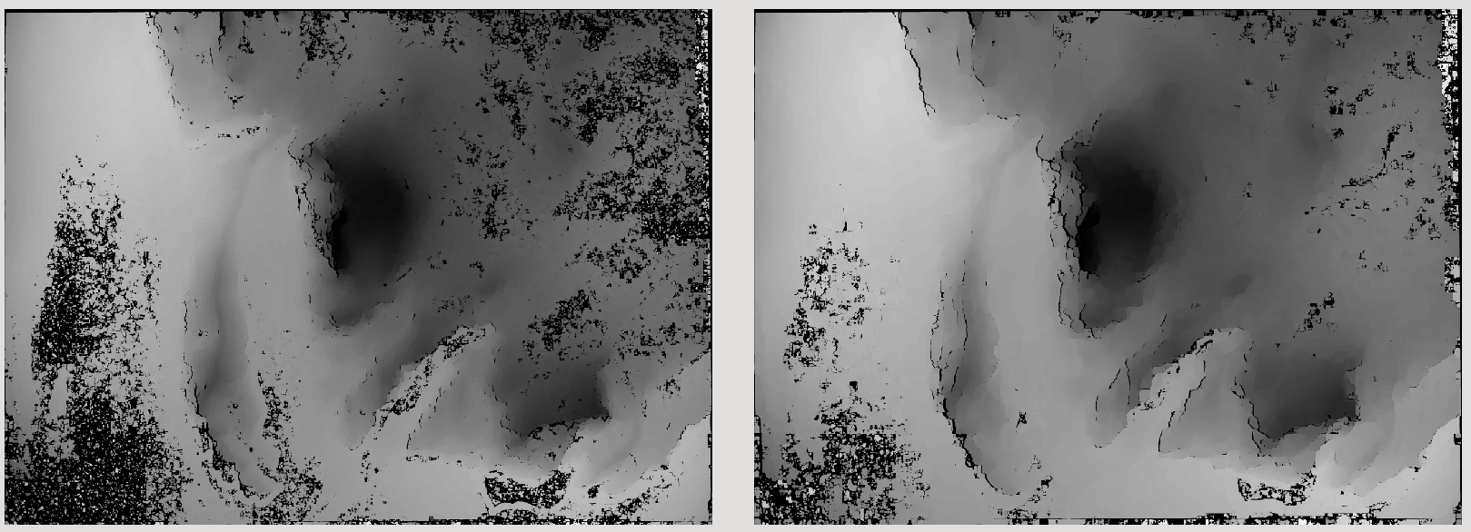
Fig. 11.4 The effect of increasing the correlation kernel size from 35 (left) to 75 (right). This location is covered in snow and several regions lack texture for the correlator to use but a large kernel increases the chances of finding useful texture for a given pixel.

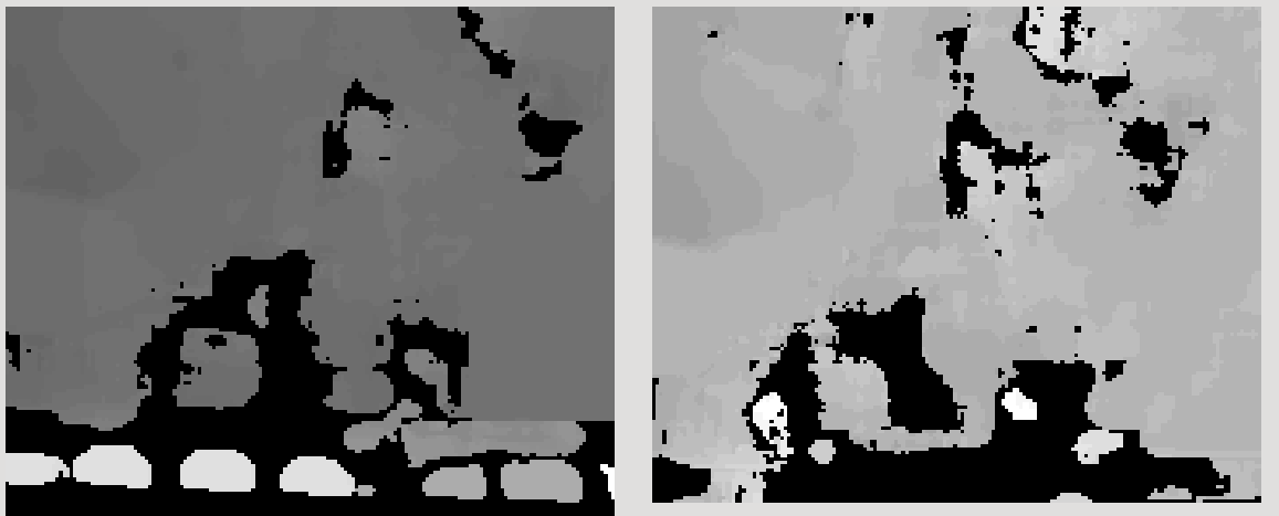
Fig. 11.5 The effect of using the rm-quantile filtering option in stereo_corr. In the left image there are a series of high disparity “islands” at the bottom of the image. In the right image quantile filtering has removed those islands while leaving the rest of the image intact.

11.4.2. Search range determination

In some circumstances, the low-resolution disparity D_sub.tif may fail to get computed, or it may be inaccurate. This can happen for example if only very small features are present in the original images, and they disappear during the resampling that is necessary to obtain D_sub.tif. In this case, it is possible to set corr-seed-mode to 0, and manually set a search range to use for full-resolution correlation via the parameter corr-search. In stereo.default (Section 17) this parameter’s entry will look like:

corr-search -80 -2 20 2

The exact values to use with this option you’ll have to discover yourself. These four numbers represent the horizontal minimum boundary, vertical minimum boundary, horizontal maximum boundary, and finally the horizontal maximum boundary within which we will search for the disparity during correlation.

It can be tricky to select a good search range. That’s why the best way is to let parallel_stereo perform an automated determination. If you think that you can do a better estimate of the search range, take look at what search ranges stereo_corr prints in the log files in the output directory, and examine the intermediate disparity images using the disparitydebug program, to figure out which search directions can be expanded or contracted. The output images will clearly show good data or bad data depending on whether the search range is correct.

The worst case scenario is to determine the search range manually. The aligned L.tif and R.tif images (Section 19) can be opened in stereo_gui (Section 16.69), and the coordinates of points that can be matched visually can be compared. Click on a pixel to have its coordinates printed in the terminal. Subtract row and column locations of a feature in the first image from the locations of the same feature in the second image, and this will yield offsets that can be used in the search range. Make several of these offset measurements (for example, for features at higher and then lower elevations), and use them to define a row and column bounding box, then expand this by 50% and use it for corr-search. This will produce good results in most cases.

If the search range produced automatically from the low-resolution disparity is too big, perhaps due to outliers, it can be tightened with either --max-disp-spread or --corr-search-limit, before continuing with full-resolution correlation (Section 17). But note that for very steep terrains and no use of mapprojection a large search range is expected, and tightening it too much may result in an inaccurate disparity.

11.5. Sub-pixel refinement

Once disparity map initialization is complete, every pixel in the disparity map will either have an estimated disparity value, or it will be marked as invalid. All valid pixels are then adjusted in the sub-pixel refinement stage based on the subpixel-mode setting.

The first mode is parabola-fitting sub-pixel refinement (subpixel-mode 1). This technique fits a 2D parabola to points on the correlation cost surface in an 8-connected neighborhood around the cost value that was the “best” as measured during disparity map initialization. The parabola’s minimum can then be computed analytically and taken as as the new sub-pixel disparity value.

This method is easy to implement and extremely fast to compute, but it exhibits a problem known as pixel-locking: the sub-pixel disparities tend toward their integer estimates and can create noticeable “stair steps” on surfaces that should be smooth [SHM06, SS03]. See for example Fig. 11.6. Furthermore, the parabola subpixel mode is not capable of refining a disparity estimate by more than one pixel, so although it produces smooth disparity maps, these results are not much more accurate than the results that come out of the disparity map initialization in the first place. However, the speed of this method makes it very useful as a “draft” mode for quickly generating a DEM for visualization (i.e. non-scientific) purposes. It is also beneficial in the event that a user will simply downsample their DEM after generation in Stereo Pipeline.

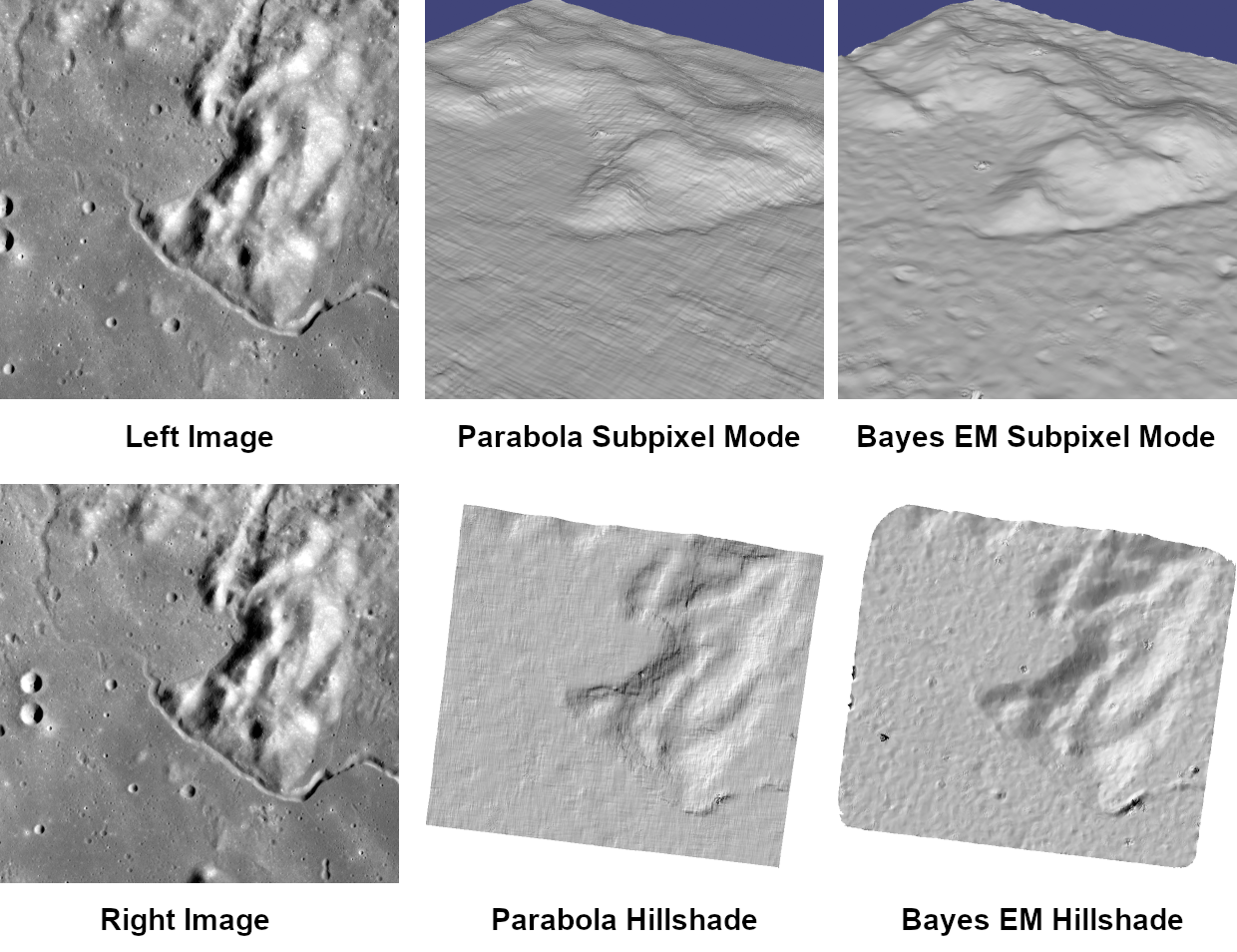
Fig. 11.6 Left: Input images. Center: results using the parabola draft subpixel mode (subpixel-mode = 1). Right: results using the Bayes EM high quality subpixel mode (subpixel-mode = 2).

For high quality results, we recommend subpixel-mode 2: the Bayes EM weighted affine adaptive window correlator. This advanced method produces extremely high quality stereo matches that exhibit a high degree of immunity to image noise. For example Apollo Metric Camera images are affected by two types of noise inherent to the scanning process: (1) the presence of film grain and (2) dust and lint particles present on the film or scanner. The former gives rise to noise in the DEM values that wash out real features, and the latter causes incorrect matches or hard to detect blemishes in the DEM. Attenuating the effect of these scanning artifacts while simultaneously refining the integer disparity map to sub-pixel accuracy has become a critical goal of our system, and is necessary for processing real-world data sets such as the Apollo Metric Camera data.

The Bayes EM subpixel correlator also features a deformable template window from the left image that can be rotated, scaled, and translated as it zeros in on the correct match in the right image. This adaptive window is essential for computing accurate matches on crater or canyon walls, and on other areas with significant perspective distortion due to foreshortening.

This affine-adaptive behavior is based on the Lucas-Kanade template tracking algorithm, a classic algorithm in the field of computer vision [BM04]. We have extended this technique; developing a Bayesian model that treats the Lucas-Kanade parameters as random variables in an Expectation Maximization (EM) framework. This statistical model also includes a Gaussian mixture component to model image noise that is the basis for the robustness of our algorithm. We will not go into depth on our approach here, but we encourage interested readers to read our papers on the topic [BNM+09, NHB+09].

However we do note that, like the computations in the disparity map initialization stage, we adopt a multi-scale approach for sub-pixel refinement. At each level of the pyramid, the algorithm is initialized with the disparity determined in the previous lower resolution level of the pyramid, thereby allowing the subpixel algorithm to shift the results of the disparity initialization stage by many pixels if a better match can be found using the affine, noise-adapted window. Hence, this sub-pixel algorithm is able to significantly improve upon the results to yield a high quality, high resolution result.

Another option when run time is important is subpixel-mode 3: the simple affine correlator. This is essentially the Bayes EM mode with the noise correction features removed in order to decrease the required run time. In data sets with little noise this mode can yield results similar to Bayes EM mode in approximately one fifth the time.

A different option is Phase Correlation, subpixel-mode 4, which implements the algorithm from [GSTF08]. It is slow and does not work well on slopes but since the algorithm is very different it might perform in situations where the other algorithms are not working well.

11.6. Triangulation

When running an ISIS session, the Stereo Pipeline uses geometric camera models available in ISIS [And08]. These highly accurate models are customized for each instrument that ISIS supports. Each ISIS “cube” file contains all of the information that is required by the Stereo Pipeline to find and use the appropriate camera model for that observation.

Other sessions such as DG (DigitalGlobe) or Pinhole, require that their camera model be provided as additional arguments to the parallel_stereo command. Those camera models come in the form of an XML document for DG and as *.pinhole, *.tsai, *.cahv, *.cahvor for Pinhole sessions. Those files must be the third and forth arguments or immediately follow after the two input images for parallel_stereo.

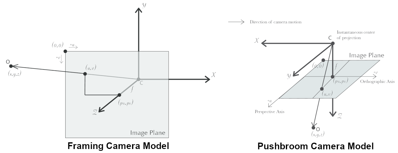
Fig. 11.7 Most remote sensing cameras fall into two generic categories based on their basic geometry. Framing cameras (left) capture an instantaneous two-dimensional image. Linescan cameras (right) capture images one scan line at a time, building up an image over the course of several seconds as the satellite moves through the sky.

ISIS camera models account for all aspects of camera geometry, including both intrinsic (i.e. focal length, pixel size, and lens distortion) and extrinsic (e.g. camera position and orientation) camera parameters. Taken together, these parameters are sufficient to “forward project” a 3D point in the world onto the image plane of the sensor. It is also possible to “back project” from the camera’s center of projection through a pixel corresponding to the original 3D point.

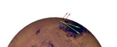
Fig. 11.8 Once a disparity map has been generated and refined, it can be used in combination with the geometric camera models to compute the locations of 3D points on the surface of Mars. This figure shows the position (at the origins of the red, green, and blue vectors) and orientation of the Mars Global Surveyor at two points in time where it captured images in a stereo pair.

Notice, however, that forward and back projection are not symmetric operations. One camera is sufficient to “image” a 3D point onto a pixel located on the image plane, but the reverse is not true. Given only a single camera and a pixel location \(x = (u,v),\) that is the image of an unknown 3D point \(P = (x,y,z)\), it is only possible to determine that \(P\) lies somewhere along a ray that emanates from the camera center through the pixel location \(x\) on the image plane (see Fig. 11.7).

Alas, once images are captured, the route from image pixel back to 3D points in the real world is through back projection, so we must bring more information to bear on the problem of uniquely reconstructing our 3D point. In order to determine \(P\) using back projection, we need two cameras that both contain pixel locations \(x_1\) and \(x_2\) where \(P\) was imaged. Now, we have two rays that converge on a point in 3D space (see Fig. 11.8). The location where they meet must be the original location of \(P\).

11.6.1. Triangulation error

In practice, the rays emanating from matching pixels in the cameras rarely intersect perfectly on the ground because any slight error in the position or pointing information of the cameras will affect the accuracy of the rays. The matching (correlation) among the images is also not perfect, contributing to the error budget. Then, we take the closest point of intersection of the two rays as the location of the intersection point \(P\).

Additionally, the actual shortest distance between the rays at this point is an interesting and important error metric that measures how self-consistent our two camera models are for this point. It will be seen in the next chapter that this information, when computed and averaged over all reconstructed 3D points, can be a valuable statistic for determining whether to carry out bundle adjustment (Section 16.5).

The distance between the two rays emanating from matching points in the cameras at their closest intersection is recorded in the fourth channel of the point cloud file, output-prefix-PC.tif. This is called the triangulation error, or the ray intersection error. It is measured in meters. This error can be gridded when a DEM is created from the point cloud by using the --errorimage argument on the point2dem command (Section 16.57).

This error is not the true accuracy of the DEM. It is only another indirect measure of quality. A DEM with high triangulation error, as compared to the ground sample distance, is always bad and should have its images bundle-adjusted. A DEM with low triangulation error is at least self-consistent, but could still be bad, or at least misaligned.

If, after bundle adjustment, the triangulation error is still high at the image corners and the inputs are Pinhole cameras, one may have to refine the intrinsics, including the distortion model. Section 12 discusses bundle adjustment, including optimizing the intrinsics.

To improve the location of a triangulated point cloud or created DEM relative to a known ground truth, use alignment (Section 16.54).

See Section 14 for another metric qualifying the accuracy of a point cloud or DEM, namely the horizontal and vertical uncertainty, as propagated from the input cameras.

11.6.2. Stereo with images mapprojected using ISIS

This is a continuation of the discussion at Section 4.2. It describes how to mapproject the input images using the ISIS tool cam2map and how to run stereo with the obtained images. Alternatively, the images can be mapprojected using ASP itself, per Section 6.1.7.

Mapprojection can result in improved results for steep slopes, when the images are taken from very different perspectives, or if the curvature of the planet/body being imaged is non-negligible.

We will now describe how this works, but we also provide the cam2map4stereo.py program (Section 16.6) which does this automatically.

The ISIS cam2map program will map-project these images:

ISIS> cam2map from=M0100115.cub to=M0100115.map.cub
ISIS> cam2map from=E0201461.cub to=E0201461.map.cub \
        map=M0100115.map.cub matchmap=true

At this stage we can run the stereo program with map-projected images:

ISIS> parallel_stereo E0201461.map.cub M0100115.map.cub   \
        --alignment-method none -s stereo.default.example \
        results/output

Here we have used alignment-method none since cam2map4stereo.py brought the two images into the same perspective and using the same resolution. If you invoke cam2map independently on the two images, without matchmap=true, their resolutions may differ, and using an alignment method rather than none to correct for that is still necessary.

Now you may skip to chapter Section 6 which will discuss the parallel_stereo program in more detail and the other tools in ASP. Or, you can continue reading below for more details on mapprojection.

11.7. Advanced discussion of mapprojection

Notice the order in which the images were run through cam2map. The first projection with M0100115.cub produced a map-projected image centered on the center of that image. The projection of E0201461.cub used the map= parameter to indicate that cam2map should use the same map projection parameters as those of M0100115.map.cub (including center of projection, map extents, map scale, etc.) in creating the projected image. By map-projecting the image with the worse resolution first, and then matching to that, we ensure two things: (1) that the second image is summed or scaled down instead of being magnified up, and (2) that we are minimizing the file sizes to make processing in the Stereo Pipeline more efficient.

Technically, the same end result could be achieved by using the mocproc program alone, and using its map= M0100115.map.cub option for the run of mocproc on E0201461.cub (it behaves identically to cam2map). However, this would not allow for determining which of the two images had the worse resolution and extracting their minimum intersecting bounding box (see below). Furthermore, if you choose to conduct bundle adjustment (see Section 12) as a pre-processing step, you would do so between mocproc (as run above) and cam2map.

The above procedure is in the case of two images which cover similar real estate on the ground. If you have a pair of images where one image has a footprint on the ground that is much larger than the other, only the area that is common to both (the intersection of their areas) should be kept to perform correlation (since non-overlapping regions don’t contribute to the stereo solution).

ASP normally has no problem identifying the shared area and it still run well. Below we describe, for the adventurous user, some fine-tuning of this procedure.

If the image with the larger footprint size also happens to be the image with the better resolution (i.e. the image run through cam2map second with the map= parameter), then the above cam2map procedure with matchmap=true will take care of it just fine. Otherwise you’ll need to figure out the latitude and longitude boundaries of the intersection boundary (with the ISIS camrange program). Then use that smaller boundary as the arguments to the MINLAT, MAXLAT, MINLON, and MAXLON parameters of the first run of cam2map. So in the above example, after mocproc with Mapping= NO you’d do this:

ISIS> camrange from=M0100115.cub
         ... lots of camrange output omitted ...
Group = UniversalGroundRange
  LatitudeType       = Planetocentric
  LongitudeDirection = PositiveEast
  LongitudeDomain    = 360
  MinimumLatitude    = 34.079818835324
  MaximumLatitude    = 34.436797628116
  MinimumLongitude   = 141.50666207418
  MaximumLongitude   = 141.62534719278
End_Group
         ... more output of camrange omitted ...

ISIS> camrange from=E0201461.cub
         ... lots of camrange output omitted ...
Group = UniversalGroundRange
  LatitudeType       = Planetocentric
  LongitudeDirection = PositiveEast
  LongitudeDomain    = 360
  MinimumLatitude    = 34.103893080982
  MaximumLatitude    = 34.547719435156
  MinimumLongitude   = 141.48853937384
  MaximumLongitude   = 141.62919740048
End_Group
         ... more output of camrange omitted ...

Now compare the boundaries of the two above and determine the intersection to use as the boundaries for cam2map:

ISIS> cam2map from=M0100115.cub to=M0100115.map.cub   \
        DEFAULTRANGE=CAMERA MINLAT=34.10 MAXLAT=34.44 \
        MINLON=141.50 MAXLON=141.63
ISIS> cam2map from=E0201461.cub to=E0201461.map.cub \
        map=M0100115.map.cub matchmap=true

You only have to do the boundaries explicitly for the first run of cam2map, because the second one uses the map= parameter to mimic the map-projection of the first. These two images are not radically different in spatial coverage, so this is not really necessary for these images, it is just an example.

Again, unless you are doing something complicated, using the cam2map4stereo.py (Section 16.6) will take care of all these steps for you.

11.7.1. Identifying issues in local alignment

Stereo with local epipolar alignment (Section 6.1) can perform better than with global affine epipolar alignment. Yet, when stereo fails on a locally aligned tile pair, it is instructive to understand why. Usually it is because the images are difficult at that location, such as due to very steep terrain, clouds, shadows, etc.

For a completed parallel_stereo run which failed in a portion, the first step is to identify the offending tile directory. For that, open the produced DEM in stereo_gui, and use the instructions at Section 16.69.8 to find the approximate longitude, latitude, and height at the problematic location.

Then run stereo_parse with the same options as parallel_stereo and the flag:

--tile-at-location '<lon> <lat> <height>'

This should print on the screen a text like:

Tile with location: run/run-2048_3072_1024_1024

If a run failed to complete, find the most recent output tile directories that were being worked on, based on modification time, and investigate one of them.

In either case, given a candidate for a problematic tile, from the log file of stereo_corr in that tile’s directory you can infer the full correlation command that failed. Re-run it, while appending the option:

--local-alignment-debug

Images and interest point matches before and after alignment will be saved. Those can be examined as:

stereo_gui <tile>-left-crop.tif <tile>-right-crop.tif \
  <tile>-left-crop__right-crop.match

and:

stereo_gui <tile>-left-aligned-tile.tif               \
  <tile>-right-aligned-tile.tif                       \
  <tile>-left-aligned-tile__right-aligned-tile.match