8.14. Kaguya Terrain Camera¶

The Kaguya Terrain Camera (TC) is a push-broom imager, with a spatial resolution of 10 m. The images are acquired from a 100 km altitude above the Moon. It was part of the JAXA Kaguya orbiter.

Kaguya TC has two sensors, named TC1 and TC2, forming a stereo pair. They see roughly the same region on the ground, with a convergence angle of about 30 degrees (Section 8.1). These sensors may have slightly different focal lengths and distortion coefficients.

8.14.1. Fetching the data¶

Visit the product search page, and enter a small search region.

Fetch the raw data sets for a desired stereo pair, starting with the TC1 and TC2 prefixes (not the DEM or other products). Both the .img and .lbl files are needed.

wget https://darts.isas.jaxa.jp/pub/pds3/sln-l-tc-3-w-level2b0-v1.0/20080605/data/TC1W2B0_01_02936N034E0938.img.gz
wget https://darts.isas.jaxa.jp/pub/pds3/sln-l-tc-3-w-level2b0-v1.0/20080605/data/TC1W2B0_01_02936N034E0938.lbl

wget https://darts.isas.jaxa.jp/pub/pds3/sln-l-tc-3-w-level2b0-v1.0/20080605/data/TC2W2B0_01_02936N036E0938.img.gz
wget https://darts.isas.jaxa.jp/pub/pds3/sln-l-tc-3-w-level2b0-v1.0/20080605/data/TC2W2B0_01_02936N036E0938.lbl

8.14.2. Preparing the data¶

Unzip the .img.gz files with gunzip.

Ensure that ISIS is installed, and that ISISROOT and ISISDATA are set, per Section 2.1.3. The Kaguya kernels can then be downloaded with the command:

$ISISROOT/bin/downloadIsisData kaguya $ISISDATA

For each image, run commands along the lines of:

$ISISROOT/bin/kaguyatc2isis                     \
  from=TC1W2B0_01_02936N034E0938.lbl            \
  to=TC1W2B0_01_02936N034E0938.cub              \
  setnullrange=NO sethrsrange=NO sethisrange=NO \
  setlrsrange=NO setlisrange=NO

$ISISROOT/bin/spiceinit from=TC1W2B0_01_02936N034E0938.cub \
    web=false attach=TRUE cksmithed=FALSE ckrecon=TRUE     \
    ckpredicted=FALSE cknadir=FALSE spksmithed=true        \
    spkrecon=TRUE spkpredicted=FALSE shape=SYSTEM          \
    startpad=0.0 endpad=0.0

Create CSM cameras (Section 8.12):

$ISISROOT/bin/isd_generate --only_naif_spice \
    TC1W2B0_01_02936N034E0938.cub            \
    -k TC1W2B0_01_02936N034E0938.cub

8.14.3. Bundle adjustment and stereo¶

Run bundle adjustment (Section 16.5) and stereo (Section 16.50):

bundle_adjust                                                   \
  TC1W2B0_01_02936N034E0938.cub TC2W2B0_01_02936N036E0938.cub   \
  TC1W2B0_01_02936N034E0938.json TC2W2B0_01_02936N036E0938.json \
  --tri-weight 0.1 --camera-weight 0.0                          \
  -o ba/run

parallel_stereo --stereo-algorithm asp_mgm --subpixel-mode 9    \
  TC1W2B0_01_02936N034E0938.cub TC2W2B0_01_02936N036E0938.cub   \
  TC1W2B0_01_02936N034E0938.json TC2W2B0_01_02936N036E0938.json \
  --bundle-adjust-prefix ba/run                                 \
  stereo/run

Run point2dem (Section 16.55) to get a DEM. Consider using the stereographic projection centered at the region of interest:

point2dem --stereographic --proj-lon 93.8 --proj-lat 3.5 \
  --tr 10 stereo/run-PC.tif

See Fig. 8.17 for a clip of the produced DEM.

It is suggested to rerun stereo with mapprojected images (Section 6.1.7), to get a higher quality output.

See Section 6 for a discussion about various speed-vs-quality choices when running stereo.

8.14.4. Alignment¶

The produced DEM can be aligned with pc_align (Section 16.52) to the LOLA RDR product.

8.14.5. Shape-from-shading with Kaguya TC¶

Here it will be illustrated how to run shape-from-shading (Section 16.64) on Kaguya TC images. First, ensure that the data are fetched and a stereo terrain is created, per Section 8.14.

Shape-from-shading expects a DEM with no holes which is also rather smooth. It should be at the same ground resolution as the input images, which in this case is 10 meters per pixel. It is best to have it in a local projection, such as stereographic.

We will modify the DEM creation command from above to use a large search radius to fill any holes:

point2dem --stereographic --proj-lon 93.8 --proj-lat 3.5 \
    --tr 10 --search-radius-factor 10 stereo/run-PC.tif

(adjust the projection center for your location).

Inspect the produced DEM stereo/run-DEM.tif in stereo_gui in hillshading mode. Any additional holes can be filled with dem_mosaic (Section 16.19.2.8).

It is also suggested to blur it a little, to make it smoother:

dem_mosaic --dem-blur-sigma 2 stereo/run-filled-dem.tif \
  -o stereo/run-blurred-dem.tif

Then crop a region with gdal_translate that has no missing data.

Mapproject (Section 16.40) onto this DEM the left and right images with the corresponding .json camera files, while using the adjustments in ba/run. Overlay the resulting georeferenced images in stereo_gui. This is a very important sanity check to ensure that the cameras are registered correctly.

Run SfS as:

parallel_sfs -i stereo/run-cropped-dem.tif \
  TC1W2B0_01_02936N034E0938.cub            \
  TC2W2B0_01_02936N036E0938.cub            \
  TC1W2B0_01_02936N034E0938.json           \
  TC2W2B0_01_02936N036E0938.json           \
  --bundle-adjust-prefix ba/run            \
  --reflectance-type 1                     \
  --blending-dist 10                       \
  --min-blend-size 50                      \
  --allow-borderline-data                  \
  --threads 4                              \
  --save-sparingly                         \
  --crop-input-images                      \
  --smoothness-weight 40000                \
  --initial-dem-constraint-weight 10       \
  --max-iterations 5                       \
  --shadow-thresholds "120 120"            \
  --tile-size 200                          \
  --padding 50                             \
  --processes 10                           \
  -o sfs/run

If there are artifacts in the produced DEM, increase the smoothness weight. But if it is too large, it may blur the produced DEM too much.

The initial and final DEM can be inspected in stereo_gui. The geodiff (Section 16.25) tool can be used to compare how much the DEM changed.

The initial DEM constraint was set rather high to ensure the DEM does not change much as result of SfS. The shadow threshold depends on the pixel values and can be very different for other images.

See, for comparison, the parameter choices made for LRO NAC (Section 13.9). That example, and that entire chapter, also has the most detailed discussion for how to run SfS, including the essential role of alignment.

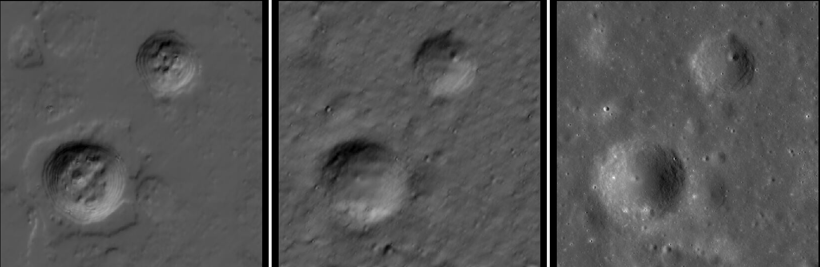
SfS with Kaguya TC images — Fig. 8.17 From left to right: the stereo DEM, SfS DEM (hillshaded), and a mapprojected image. Some numerical noise is still seen, which can be removed by increasing the smoothing weight. See below for another example.¶

Using multiple images with diverse illumination results in more detail and fewer artifacts. For such data, bundle adjustment and pairwise stereo need to be run first, and the produced DEMs and cameras must be aligned to a common reference, such as LOLA (Section 16.52.14). Then the aligned DEMs are inspected and merged with dem_mosaic, a clip is selected, holes are filled, noise is blurred, and SfS is run. The process is explained in detail in Section 13.9.

Here is an example of running SfS with the datasets:

TC{1,2}W2B0_01_02921S050E1100
TC{1,2}W2B0_01_05936S048E1097

All four images were used, though likely the first of each pair would have been sufficient, given that images in each pair have the same illumination.

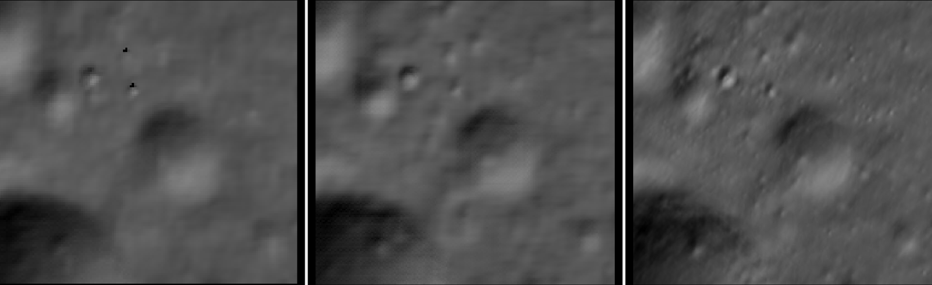
SfS with Kaguya TC images with different illumination — Fig. 8.18 SfS with Kaguya images with different illumination. From left to right: first pair stereo DEM, second pair stereo DEM, and the SfS DEM (all hillshaded). It can be seen that SfS adds more detail and removes numerical noise.¶

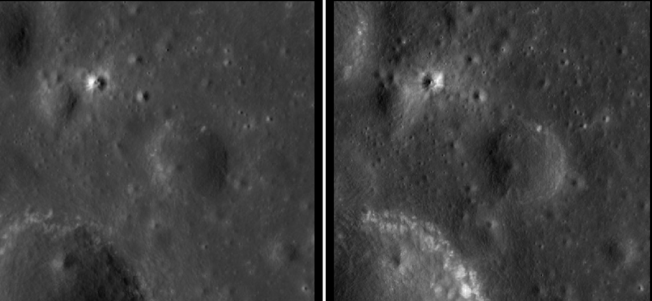
SfS Kaguya TC ortho images — Fig. 8.19 The images used for SfS (one from each pair). The Sun is in the East and West, respectively.¶

8.14.6. Refining the camera intrinsics for Kaguya TC¶

See Section 12.2.2.