8.27. Shallow-water bathymetry

ASP supports creation of terrain models where parts of the terrain are under water. Assuming that the water is shallow, still, clear, with sufficient texture to match at the water bottom between the left and right images, the rays emanating from the cameras and converging at those features will be bent according to Snell’s law at the water interface, hence determining correctly the position of underwater terrain.

The bathymetry module is evaluated in [PAD21] and [PLADS23].

8.27.1. Software considerations

ASP supports the bathymetry mode only with the dg, rpc, and nadirpinhole sessions, so with Digital Globe linescan cameras, RPC cameras, and pinhole cameras (Section 8.27.14), all for Earth. Both raw and mapprojected images can be used (Section 8.27.12), with or without bundle adjustment or alignment (Section 8.27.8).

8.27.2. Physics considerations

Shallow water does not appear equally transparent at all wavelengths, which will affect the quality of the results. While the process we outline below will work, in principle, with any data, we will focus on stereo with the G band (green, stored at band 3) of Digital Globe multispectral imagery, and we will use the N band (near-infrared 1, stored at band 7), to determine a mask of the ground vs water.

These or any other bands can be extracted from a multi-band image as follows:

b=3
gdal_translate -b ${b} -co compress=lzw -co TILED=yes \
  -co BLOCKXSIZE=256 -co BLOCKYSIZE=256               \
  input.TIF input_b${b}.tif

The extra options, in addition to -b ${b} to extract a given band, are needed to create a compressed and tiled output image, which helps with the performance of ASP later.

8.27.3. Computation of the water-land threshold

In order to distinguish points on land from those under water, a mask needs to be computed for each of the left and right input images, with the masks having the same dimensions as those images.

A simple way of creating such a mask is to first determine a threshold such that pixels at or below threshold are under water, and those above threshold are on land.

It was experimentally found that it is best to use band 7 (near infrared) for Digital Globe multispectral images to find this water threshold, as in them the water appears universally darker than the land.

ASP provides two tools for finding the threshold in automated way based on histogram analysis. One is bathy_threshold_calc.py (Section 16.4), and the second one is otsu_threshold (Section 16.46). This last tool produces a somewhat higher threshold compared to the other one, but in practice the results with both approaches are very similar.

The bathy_threshold_calc.py program works based on the observation that, since in such an image the water appears darker than the land, then in a histogram of the pixels in the image, the water and land appear as two noticeable peaks, with a good value for the threshold then being the image value at the bottom of the valley between those peaks.

For robustness to noise, this histogram is approximated by a kernel-density estimate (KDE) using Gaussian kernels. It is very important to note that even then this tool may return the wrong minimum, which it assumes to be the first one.

Therefore, this tool plots the histogram, its kernel density estimate, the positions of the minima, and prints their locations on screen. The user is responsible for validating visually where the most appropriate position of the minimum is (along the horizontal axis).

The kernel-density estimate calculation is very time-consuming for large images, hence it is suggested to pass to the tool the number of samples to use (it will pick the samples uniformly in the image). For example, if a million samples are used, the calculation should take a few minutes to complete.

This program can be invoked for each of the left and right images as follows:

~/miniconda3/envs/bathy/bin/python $(which bathy_threshold_calc.py) \
  --image left.tif --num-samples 1000000

Here it is assumed that ASP’s bin directory is in the path. The bathy conda environment should be installed as described in Section 16.4.

It is suggested to experiment a bit with the number of samples, using, for example, double of this amount, and see the difference. Normally the outcome should be rather similar.

It will produce the following output:

Image file is left.tif
Number of samples is 1000000
Number of image rows and columns: 7276, 8820
Picking a uniform sample of dimensions 908, 1101
Please be patient. It make take several minutes to find the answer.
Positions of the minima:  [ 155.18918919  802.7027027 ... ]
Suggested threshold is the position of the first minimum:  155.1891891891892
Please verify with the graph. There is a chance the second minimum may work better.
Elapsed time in seconds: 275.2

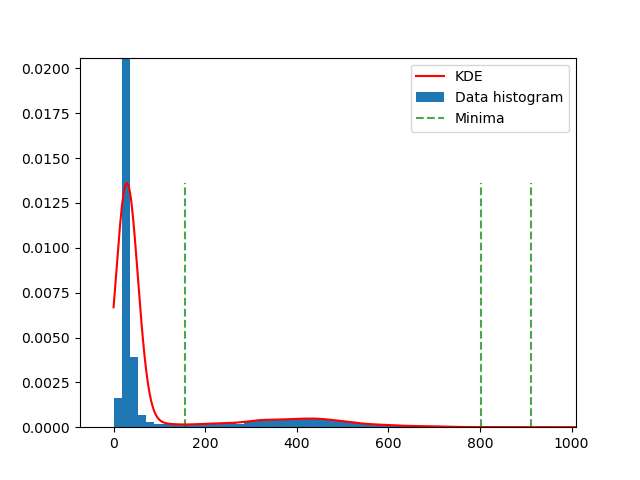
Fig. 8.25 Example of the graph plotted by bathy_threshold_calc.py

Once the threshold is found, stereo_gui can be used to visualize the regions at or below threshold (Section 16.67.14).

8.27.4. Creation of masks based on the threshold

Having determined the water-land threshold, the left and right image masks will be found from the corresponding images as follows:

left_thresh=155.1891891891892
image_calc -c "max($left_thresh, var_0)" -d float32 \
  --output-nodata-value $left_thresh                \
  left_b7.tif -o left_mask.tif

Here, left_b7.tif is suggestive of the fact that the band 7 of WorldView multispectral imagery was used.

It is important to remember to use the right image threshold when repeating this process for the right image.

This tool sets the pixel values at or below threshold to the no-data value, while keeping unchanged the values above the threshold.

Later, when doing stereo, if, based on the masks, a pixel in the left image is under water, while the corresponding pixel in the right image is not, for noise or other reasons, that pixel pair will be declared to be on land and hence no bathymetry correction will take place for this pair. Hence, some inspection and potentially cleanup of the masks may be necessary.

8.27.5. Determination of the water surface

In order to run stereo and properly triangulate the rays which may intersect under water, it is necessary to determine the water surface. Since for images of large extent the Earth curvature will be important, this surface will be found as a plane in a local stereographic projection.

The procedure for this is described in Section 16.3.

8.27.6. Stereo with bathymetry correction

Having these in place, stereo can then happen as follows:

parallel_stereo -t dg left.tif right.tif left.xml right.xml \
  --left-bathy-mask left_mask.tif                           \
  --right-bathy-mask right_mask.tif                         \
  --stereo-algorithm asp_mgm                                \
  --refraction-index 1.34 --bathy-plane bathy_plane.txt     \
  run_bathy/run

Here we specified the two masks, the water index of refraction, and the water plane found before.

See Section 6 for a discussion about various speed-vs-quality choices.

This is followed by creating a DEM:

point2dem run_bathy/run-PC.tif --orthoimage run_bathy/run-L.tif

The water refraction index was set 1.34 [Jer76]. Alternatively, one could use 1.333 [HS98, ThormahlenSG85], or a more precise value that depends on wavelength, temperature, and if having saltwater or freshwater (Parrish (2020), [AH76, Mob95]). For example, using the equation and coefficients found in Parrish (2020), and the green wavelength for saltwater, the water refraction index is 1.340125 when the water temperature is 27 ° C (this was applied to a Florida Keys test site for the month of May).

The obtained point cloud will have both triangulated points above water, so with no correction, and below water, with the correction applied. If desired to have only one of the two, call the parallel_stereo command with the option --output-cloud-type with the value topo or bathy respectively (the default for this option is all).

The bathymetry correction happens at the triangulation stage (though the necessary transformations on the bathymetry masks are done in pre-processing). Hence, after a stereo run finished, it is only necessary to re-run the stereo_tri step if desired to apply this correction or not, or if to change the value of --output-cloud-type.

As in usual invocations of stereo, the input images may be mapprojected, and then a DEM is expected, stereo may happen only in certain regions as chosen in the GUI, bundle adjustment may be used, the output point cloud may be converted to LAS, etc.

8.27.7. Performing sanity checks on a bathy run

The results produced with the bathymetry mode for stereo need careful validation. Here we will show how to examine if the water-land boundary and corresponding water surface were found correctly.

Before that, it is important to note that such runs can take a long time, and one should try to first perform a bathymetry experiment in a carefully chosen small area by running stereo_gui instead of parallel_stereo, while keeping the rest of the bathy options as above, and then selecting clips in the left and right images with the mouse to run parallel_stereo on. See Section 16.67 for more info.

If the bathy_plane_calc is run with the option:

--output-inlier-shapefile inliers.shp

it will produce a shapefile for the inliers.

Create an orthoimage from the aligned bathy mask, for example, such as:

point2dem --no-dem run_bathy/run-PC.tif                \
  --orthoimage run_bathy/run-L_aligned_bathy_mask.tif  \
  -o run_bathy/run-bathy_mask

This should create run_bathy/run-bathy_mask-DRG.tif.

This should be overlayed in stereo_gui on top of the inliers from the bathy plane calculation, as:

stereo_gui --single-window --use-georef inliers.shp    \
  run_bathy/run-bathy_mask-DRG.tif

The inliers should be well-distributed on the land-water interface as shown by the mask.

To verify that the water surface was found correctly, one can create a DEM with no bathymetry correction, subtract from that one the DEM with bathymetry correction, and colorize the result. This can be done by redoing the triangulation in the previous run, this time with no bathy information:

mv run_bathy/run-DEM.tif run_bathy/run-yesbathy-DEM.tif
parallel_stereo -t dg left.tif right.tif left.xml right.xml \
  --stereo-algorithm asp_mgm                                \
  --entry-point 5 run_bathy/run
point2dem run_bathy/run-PC.tif -o run_bathy/run-nobathy

Note that we started by renaming the bathy DEM. The result of these commands will be run_bathy/run-nobathy-DEM.tif. The differencing and colorizing is done as:

geodiff run_bathy/run-nobathy-DEM.tif             \
  run_bathy/run-yesbathy-DEM.tif -o run_bathy/run
colormap --min 0 --max 1 run_bathy/run-diff.tif

The obtained file, run_bathy/run-diff_CMAP.tif, can be added to the stereo_gui command from above. Colors hotter than blue will be suggestive of how much the depth elevation changed as result of bathymetry correction. It is hoped that no changes will be seen on land, and that the inliers bound well the region where change of depth happened.

8.27.8. Bundle adjustment and alignment

It is important to note that we did not use bundle adjustment (Section 16.5) or pc_align (Section 16.52) for alignment. That is possible, but then one has to ensure that all the data are kept consistent under such operations.

In particular, running bundle adjustment on a PAN image pair, and then on a corresponding multispectral band pair, will result in DEMs which are no longer aligned either to each other, or to their versions before bundle adjustment. The cameras can be prevented by moving too far if bundle_adjust is called with, for example, --tri-weight 0.1, or some other comparable value, to constrain the triangulated points. Yet, by its very nature, this program changes the positions and orientations of the cameras, and therefore the coordinate system. And note that a very high camera weight may interfere with the convergence of bundle adjustment.

It is suggested to use these tools only if a trusted reference dataset exists, and then the produced DEMs should be aligned to that dataset.

Only the “topo” component of a DEM obtained with ASP should be used for alignment (see --output-cloud-type), that is, the part above water, as the part under water can be quite variable given the water level. Here’s an example for creating the “topo” DEM, just the triangulation stage processing needs modification:

 parallel_stereo -t dg left.tif right.tif left.xml right.xml \
   --stereo-algorithm asp_mgm                                \
   <other options>                                           \
   --entry-point 5 --output-cloud-type topo                  \
     run_bathy/run
point2dem run_bathy/run-PC.tif -o run_bathy/run-topo

which will create run_bathy/run-topo-DEM.tif.

Then, after the “topo” DEM is aligned, the alignment transform can be applied to the full DEM (obtained at triangulation stage with --output-cloud-type all), as detailed in Section 16.52.6. The input cameras can be aligned using the same transform (Section 16.52.14).

When the water surface is determined using a DEM, a mask of the image portion above water, and corresponding camera, and the cameras have been bundle-adjusted or aligned, the option --bundle-adjust-prefix must be used with bathy_plane_calc (see Section 16.3.1).

8.27.9. Validation of alignment

It is very strongly suggested to use visual inspection in stereo_gui and the geodiff and colormap tools for differencing DEMs to ensure DEMs that are meant to be aligned have small differences. Since bathymetry modeling can measure only very shallow water depths, any misalignment can result in big errors in final results.

If DEMs have parts under water and it is desired to remove those for the purpose of alignment, one can take advantage of the fact that the water height is roughly horizontal. Hence, a command like:

height=-21.2
image_calc -c "max($height, var_0)" -d float32 \
  --output-nodata-value $height                \
  dem.tif -o topo_dem.tif

will eliminate all heights under -21.2 meters (relative to the datum ellipsoid).

8.27.10. Bathymetry with changing water level

If the left and right images were acquired at different times, the water level may be different among the two, for example because of the tide. Then, bathy_plane_calc (Section 16.3) can be used independently for the left and right images, obtaining two such surfaces. These can be passed to ASP as follows:

parallel_stereo --bathy-plane "left_plane.txt right_plane.txt" \
  --stereo-algorithm asp_mgm                                   \
  <other options>

The computation will go as before until the triangulation stage. There, the rays emanating from the cameras will bend when meeting the water at different elevations given by these planes, and their intersection may happen in three possible regimes (above both planes, in between them, or below both of them).

Care must be taken when doing stereo with images acquired at a different times as the illumination may be too different. A good convergence angle is also expected (Section 8.1).

8.27.11. How to reuse most of a run

Stereo can take a long time, and the results can have a large size on disk. It is possible to reuse most of such a run, using the option --prev-run-prefix, if cameras or camera adjustments (option --bundle-adjust-prefix) get added, removed, or change, if the water surface (--bathy-plane) or index of refraction change, or if the previous run did not do bathy modeling but the new run does (hence the options --left-bathy-mask and --right-bathy-mask got added).

One must not change --left-image-crop-win and --right-image-crop-win in the meantime, if used, as that may invalidate the intermediate files we want to reuse, nor the input images. If the previous run did employ bathy masks, and it is desired to change them (rather than add them while they were not there before), run the touch command on the new bathy masks, to give the software a hint that the alignment of such masks should be redone.

As an example, consider a run with no bathymetry modeling:

parallel_stereo -t dg left.tif right.tif left.xml right.xml \
  --stereo-algorithm asp_mgm                                \
  run_nobathy/run

A second run, with output prefix run_bathy/run, can be started directly at the triangulation stage while reusing the earlier stages from the other run as:

parallel_stereo -t dg left.tif right.tif left.xml right.xml         \
  --stereo-algorithm asp_mgm                                        \
  --left-bathy-mask left_mask.tif --right-bathy-mask right_mask.tif \
  --refraction-index 1.34 --bathy-plane bathy_plane.txt             \
  --bundle-adjust-prefix ba/run run_yesbathy/run                    \
  --prev-run-prefix run_nobathy/run

The explanation behind the shortcut employed above is that the precise cameras and the bathy info are fully used only at the triangulation stage. That because the preprocessing step (step 0), mostly does alignment, for which some general knowledge of the cameras and bathy information is sufficient, and other steps, before triangulation, work primarily on images. This option works by making symbolic links to files created at previous stages of stereo which are needed at triangulation.

Note that if the cameras changed, the user must recompute the bathy planes first, using the updated cameras. The bathy_plane_calc tool which is used for that can take into account the updated cameras via the --bundle-adjust-prefix option passed to it.

If the software notices that the current run invoked with --prev-run-prefix employs bathy masks, unlike that previous run, or that the modification time of the bathy masks passed in is newer than of files in that run, it will ingest and align the new masks before performing triangulation.

8.27.12. Bathymetry correction with mapprojected images

Mapprojecting the input images can improve the results on steep slopes (Section 6.1.7). While that may not be a big concern in bathymetry applications, this section nevertheless illustrates how stereo with shallow water can be done with mapprojection.

Given an external DEM, the left and right images can be mapprojected onto this DEM, for example as:

mapproject external_dem.tif --tr gridSize \
  left.tif left.xml left_map.tif

and the same for the right image. The same ground sample distance (resolution) must be used for left and right images, which should be appropriately chosen depending on the data (Section 6.1.7.4).

One should mapproject the same way the left and right band 7 Digital Globe multispectral images (if applicable), obtaining two images, left_map_b7.tif and right_map_b7.tif. These two can be used to find the masks, as earlier:

left_thresh=155.1891891891892
image_calc -c "max($left_thresh, var_0)" \
  --output-nodata-value $left_thresh     \
  left_map_b7.tif -o left_map_mask.tif

(and the same for the right image.)

The threshold determined with the original non-mapprojected images should still work, and the same water plane can be used.

Then, stereo happens as above, with the only differences being the addition of the external DEM and the new names for the images and the masks:

parallel_stereo -t dg left_map.tif right_map.tif   \
  left.xml right.xml                               \
  --stereo-algorithm asp_mgm                       \
  --left-bathy-mask left_map_mask.tif              \
  --right-bathy-mask right_map_mask.tif            \
  --refraction-index 1.34                          \
  --bathy-plane bathy_plane.txt                    \
  run_map/run external_dem.tif

8.27.13. Using Digital Globe PAN images

The bathymetry mode can be used with Digital Globe PAN images as well, though likely the water bottom may not be as transparent in this case as for the Green band.

Yet, if desired to do so, a modification is necessary if the mask for pixels above water is obtained not from the PAN image itself, but from a band of the corresponding multispectral image, because those are acquired with different sensors.

Starting with a multispectral image mask, one has to first increase its resolution by a factor of 4 to make it comparable to the PAN image, then crop about 50 columns on the left, and further crop or extend the scaled mask to match the PAN image dimensions.

ASP provides a tool for doing this, which can be called as:

scale_bathy_mask.py ms_mask.tif pan_image.tif output_pan_mask.tif

Any warnings about srcwin ... falls partially outside raster extent should be ignored. GDAL will correctly pad the scaled mask with no-data values if it has to grow it to match the PAN image.

To verify that the PAN image and obtained scaled PAN mask agree, overlay them in stereo_gui, by choosing from the top menu the option View->Single window.

It is not clear if the number of columns to remove on the left should be 50 or 48 pixels. It appears that 50 pixels works better for WV03 while 48 pixels may be appropriate for WV02. These were observed to result in a smaller shift among these images. The default is 50. If desired to experiment with another amount, pass that one as an additional argument to the tool, after the output PAN mask.

8.27.14. Using non-Digital Globe images

Stereo with bathymetry was tested with RPC cameras. In fact, the above examples can be re-run by just replacing dg with rpc for the -t option. (It is suggested that the shoreline shapefile and the water plane be redone for the RPC case. It is expected that the results will change to a certain extent.)

Experiments were also done with pinhole cameras (using the nadirpinhole session) with both raw and mapprojected images, and using the alignment methods ‘epipolar’, ‘affineepipolar’, ‘homography’, and ‘none’, giving plausible results.

8.27.15. Effect of bathymetry correction on the output DEM

It is instructive to compare the DEMs with and without the bathymetry correction.

The bathymetry correction results in the points in the output triangulated cloud being pushed “down”, as the rays emanating from the cameras become “steeper” after meeting the water.

Yet, a DEM is obtained by binning and doing weighted averaging of the points in the cloud. It can happen that with the bathymetry correction on, a point may end up in a different bin than with it off, with the result being that a handful of heights in the bathymetry-corrected DEM can be slightly above the same heights in the DEM without the correction, which is counter-intuitive.

This however will happen only close to the water-land interface and is an expected gridding artifact. (A different DEM grid size may result in the artifacts changing location and magnitude.)