9.3. MSL navcam example

This is an example of using the ASP tools to process images taken by the Mars Science Laboratory (MSL) rover Curiosity. See Section 9 for other examples.

This approach uses the images to create a self-consistent solution, which can be registered to the ground (Section 9.3.9).

Section Section 8.12.5 discusses using the known camera poses for MSL.

9.3.1. Illustration

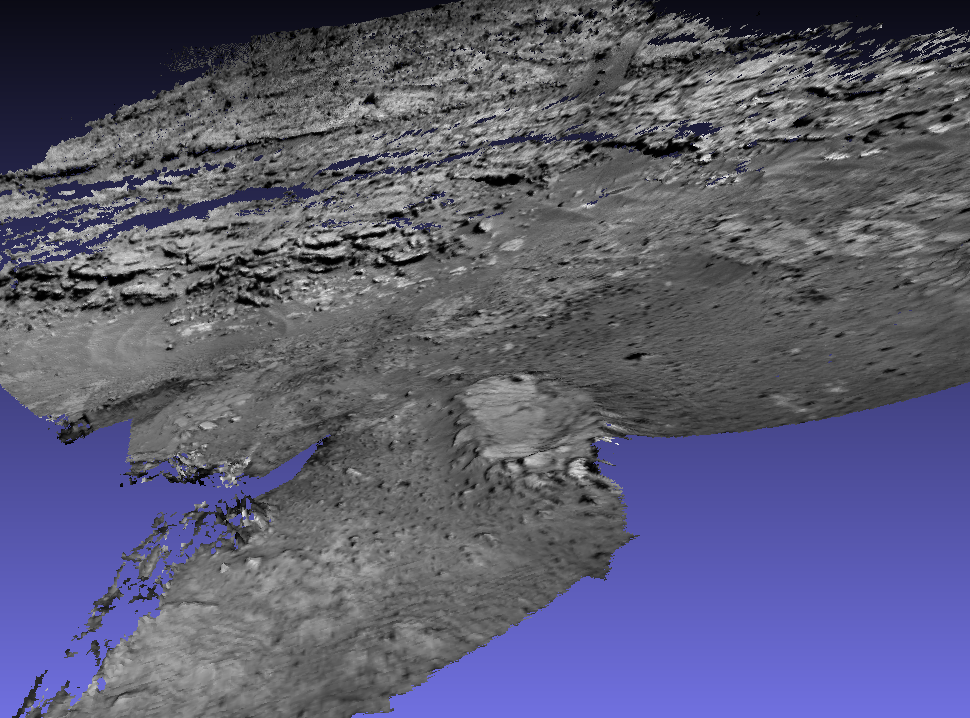
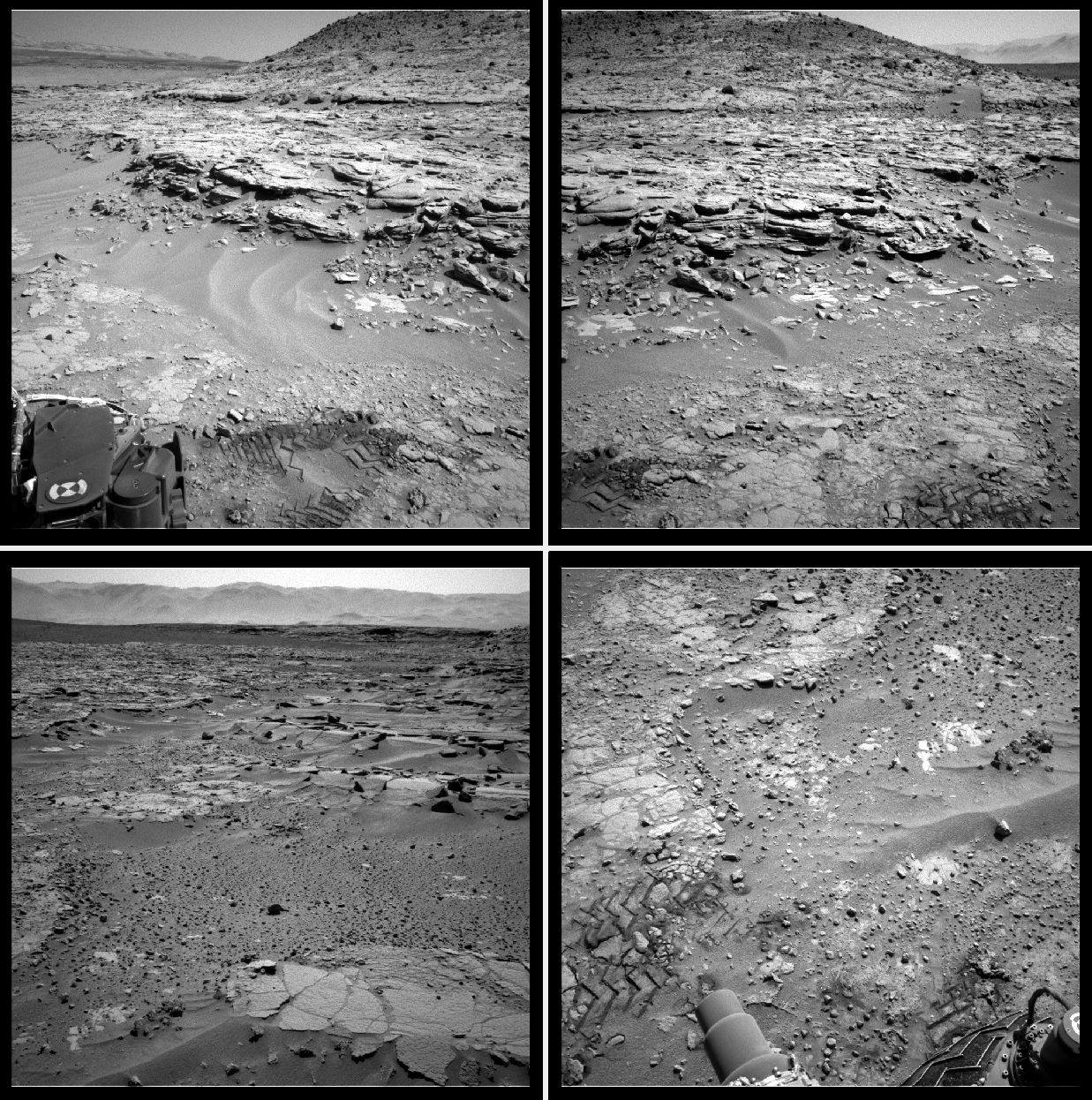
Fig. 9.2 A mesh created with 22 MSL navcam images acquired on SOL 597 (top), and several representative images from this set (bottom).

9.3.2. Sensor information

Curiosity has two navcam sensors (left and right) mounted on a stereo rig. Each records images at a resolution of 1024 x 1024 pixels. The field of view is 45 degrees.

9.3.3. Challenges

The navcam images are used to plan the path of the rover. They are not acquired specifically for mapping. While there is good overlap and perspective difference between images that are taken at the same time with the stereo rig, these assumptions may not hold for images produced at different times. Moreover, after the rover changes position, there is usually a large perspective difference and little overlap with earlier images.

A very useful reference on processing MSL images is [CLMouelicM+20]. It uses the commercial Agisoft Photoscan software. To help with matching the images, that paper uses the global position and orientation of each image and projects these onto the ground. Such data is not fully present in the .LBL files in PDS, as those contain only local coordinates, and would necessitate queering the SPICE database. It also incorporates lower-resolution “TRAV” images to tie the data together.

In the current example only a small set of data from a single day is used.

9.3.4. Data preparation

The images are fetched from PDS. For example, to get the data for day (SOL) 597 on Mars, use the command:

dir=data/msl/MSLNAV_0XXX/DATA/SOL00597
wget -r -nH --cut-dirs=4 --no-parent    \
  --reject="index.html*"                \
  https://pds-imaging.jpl.nasa.gov/$dir \
  --include $dir

This will create the directory SOL00597 containing .IMG data files and .LBL metadata. Using the ISIS pds2isis program (see Section 2.1.3 for installation), these can be converted to .cub files as:

pds2isis from = SOL00597/image.LBL to = SOL00597/image.cub

A .cub file obtained with the left navcam sensor will have a name like:

SOL00597/NLB_451023553EDR_F0310946NCAM00492M1.cub

while for the right sensor the prefix will be instead NRB. The full-resolution images have _F as part of their name, as above.

We will convert the .cub files to the PNG format so that they can be understood by image-processing programs. The rig_calibrator convention will be used, of storing each sensor’s data in its own subdirectory (Section 16.58.2). We will name the left and right navcam sensors lnav and rnav. Then, the conversion commands are along the lines of:

mkdir -p SOL00597/lnav
isis2std from = SOL00597/left_image.cub \
  to = SOL00597/lnav/left_image.png

9.3.5. Image selection

A subset of 22 images was selected for SOL 597 (half for each of the left and right navcam sensors). Images were chosen based on visual inspection. A fully automatic approach may be challenging (Section 9.3.3).

This dataset is available for download.

9.3.6. Setting up the initial rig

Given the earlier sensor information, the focal length can be found using the formula:

\[f = \frac{w}{2\tan(\frac{\theta}{2})}\]

where \(w\) is sensor width in pixels and \(\theta\) is the field of view. The focal length is then about 1236.0773 pixels. We will start by assuming that the optical center is at the image center, and no distortion. Hence, the initial rig configuration (Section 16.58.5) will look like:

ref_sensor_name: lnav

sensor_name: lnav
focal_length:  1236.0773
optical_center: 512 512
distortion_coeffs:
distortion_type: no_distortion
image_size: 1024 1024
distorted_crop_size: 1024 1024
undistorted_image_size: 1024 1024
ref_to_sensor_transform: 1 0 0 0 1 0 0 0 1 0 0 0
depth_to_image_transform: 1 0 0 0 1 0 0 0 1 0 0 0
ref_to_sensor_timestamp_offset: 0

with an additional identical block for the rnav sensor (without ref_sensor_name).

9.3.7. SfM map creation

Given the data and rig configuration, the image names in .png format were put in a list, with one entry per line. The theia_sfm program (Section 16.69) was run to find initial camera poses:

theia_sfm                     \
  --rig_config rig_config.txt \
  --image_list list.txt       \
  --out_dir theia_rig

Next, rig_calibrator (Section 16.58) is used, to enforce the rig constraint between the left and right navcam sensors and refine the intrinsics:

params="focal_length,optical_center"
float="lnav:${params} rnav:${params}"

rig_calibrator                        \
  --rig_config rig_config.txt         \
  --nvm theia_rig/cameras.nvm         \
  --camera_poses_to_float "lnav rnav" \
  --intrinsics_to_float "$float"      \
  --num_iterations 100                \
  --calibrator_num_passes 2           \
  --num_overlaps 5                    \
  --out_dir rig_out

To optimize the distortion, one can adjust the rig configuration by setting initial distortion values and type:

distortion_coeffs: 1e-8 1e-8 1e-8 1e-8 1e-8
distortion_type: radtan

and then defining the list of parameters to optimize as:

params="focal_length,optical_center,distortion"

For this example, plausible solutions were obtained with and without using distortion modeling, but likely for creation of pixel-level registered textured meshes handling distortion is important.

The produced pairwise matches in rig_out/cameras.nvm can be inspected with stereo_gui (Section 16.67.9.4).

9.3.8. Mesh creation

Here, a point cloud is created from every stereo pair consisting of a left sensor image and corresponding right image, and those are fused into a mesh. Some parameters are set up first.

Stereo options (Section 17):

stereo_opts="
  --stereo-algorithm asp_mgm
  --alignment-method affineepipolar
  --ip-per-image 10000
  --min-triangulation-angle 0.1
  --global-alignment-threshold 5
  --session nadirpinhole
  --no-datum
  --corr-seed-mode 1
  --max-disp-spread 300
  --ip-inlier-factor 0.4
  --nodata-value 0"

Point cloud filter options (Section 16.53):

maxDistanceFromCamera=100.0
pc_filter_opts="
  --max-camera-ray-to-surface-normal-angle 85
  --max-valid-triangulation-error 10.0
  --max-distance-from-camera $maxDistanceFromCamera
  --blending-dist 50 --blending-power 1"

Mesh generation options (Section 16.72):

mesh_gen_opts="
  --min_ray_length 0.1
  --max_ray_length $maxDistanceFromCamera
  --voxel_size 0.05"

Set up the pairs to run stereo on:

outDir=stereo
mkdir -p ${outDir}
grep lnav list.txt > ${outDir}/left.txt
grep rnav list.txt > ${outDir}/right.txt

The optimized rig, in rig_out/rig_config.txt, and optimized cameras, in rig_out/cameras.txt, are passed to multi_stereo (Section 16.41):

multi_stereo                              \
  --rig_config rig_out/rig_config.txt     \
  --camera_poses rig_out/cameras.txt      \
  --undistorted_crop_win '1100 1100'      \
  --rig_sensor "lnav rnav"                \
  --first_step stereo                     \
  --last_step mesh_gen                    \
  --stereo_options "$stereo_opts"         \
  --pc_filter_options "$pc_filter_opts"   \
  --mesh_gen_options "$mesh_gen_opts"     \
  --left ${outDir}/left.txt               \
  --right ${outDir}/right.txt             \
  --out_dir ${outDir}

This created:

${outDir}/lnav_rnav/fused_mesh.ply

See the produced mesh in Section 9.3.1.

9.3.9. Ground registration

To create DEMs, for example for rover cameras, the cameras should be registered to the ground. We will discuss how to do that both when a prior DEM is available and when not. For registration to a local Cartesian coordinate system, see instead Section 16.58.9.

9.3.9.1. Invocation of bundle adjustment

The rig_calibrator option --save_pinhole_cameras can export the camera poses to Pinhole format (Section 20.1). It will also save the list of input images (Section 16.58.13).

These can be ingested by ASP’s bundle adjustment program (Section 16.5). It can transform the cameras to ground coordinates using ground control points (GCP, Section 16.5.9), with the option --transform-cameras-with-shared-gcp.

Here is an example invocation:

bundle_adjust                            \
--image-list rig_out/image_list.txt      \
--camera-list rig_out/camera_list.txt    \
--nvm rig_out/cameras.nvm                \
--num-iterations 0                       \
--inline-adjustments                     \
--datum D_MARS                           \
--remove-outliers-params "75 3 50 50"    \
--transform-cameras-with-shared-gcp      \
gcp1.gcp gcp2.gcp gcp3.gcp               \
-o ba/run

The --datum option is very important, and it should be set depending on the planetary body.

Using zero iterations will only apply the registration transform, and will preserve the rig structure, up to a scale factor.

With a positive number of iterations, the cameras will be further refined in bundle adjustment, while using the GCP. For such refinement it is important to have many interest point matches between the images. This will not preserve the rig structure.

We used high values in --remove-outliers-params to avoid removing valid features in the images if there is unmodeled distortion.

See Section 16.5.11.5 for a report file that measures reprojection errors, including for GCP. It is very important to examine those. They should be less than a few dozen pixels, and ideally less.

With the cameras correctly registered and self-consistent, dense stereo point clouds and DEMs can be created (Section 6), that can be mosaicked (Section 16.19) and aligned to a prior dataset (Section 16.52).

For difficult areas with few interest points matches, the images (with cameras now in planetary coordinates) can be mapprojected, and the resulting images can be used to find many more interest points (Section 16.67.13).

9.3.9.2. Use of registered data with rig_calibrator

The bundle_adjust program will produce the file ba/run.nvm having the registered camera positions and the control network. This can be passed back to rig_calibrator, if needed, together with the latest optimized rig, which is at rig_out/rig_config.txt. The command is:

rig_calibrator                        \
  --rig_config rig_out/rig_config.txt \
  --nvm ba/run.nvm                    \
  --camera_poses_to_float "lnav rnav" \
  --intrinsics_to_float "$float"      \
  --num_iterations 100                \
  --calibrator_num_passes 2           \
  --num_overlaps 0                    \
  --out_dir rig_out_reg

Here we set --num_overlaps 0 as we do not want to try to create interest point matches again.

9.3.9.3. GCP and custom DEM creation

GCP files can be created manually by point-and-click in stereo_gui (Section 16.67.12) or automatically (Section 16.23), if a prior DEM and/or orthoimage are available.

If no prior DEM is available, it is possible to tie several features in the images to made-up ground points. For example, consider a ground box with given width and height, in meters, such as 10 x 4 meters. Create a CSV file named ground.csv of the form:

# x (meters) y(meters) height (meters)
0 0 0
10 0 0
10 4 0
0 4 0

This can be made into a DEM with point2dem (Section 16.55):

proj="+proj=stere +lat_0=0 +lat_ts=0 +lon_0=0 +k=1 +x_0=0 +y_0=0 +a=3396190 +b=3396190 +units=m +no_defs"
format="1:northing,2:easting,3:height_above_datum"
point2dem                    \
  --datum D_MARS             \
  --csv-format "$format"     \
  --csv-proj4  "$proj"       \
  --t_srs "$proj"            \
  --tr 0.1                   \
  --search-radius-factor 0.5 \
  ground.csv

Ensure the correct planet radii and datum are used.

Then, following the procedure Section 16.67.12, features can be picked in the images and tied to some of the corners of this box, creating GCP files, which are then used as earlier.

Multiple subsets of the images can be used, with each producing a GCP file. All can then be passed together to bundle_adjust.

9.3.10. Validation

Solving for both intrinsics and camera poses is a complex nonlinear problem, that may have more than one solution. It is strongly suggested to compare the produced individual DEMs (after alignment, Section 16.52) to a trusted DEM, even if at a lower resolution.

In case of horizontal misalignment, it is suggested to individually align the produced DEMs to the prior DEM, apply the alignment transform to the cameras (Section 16.52.14), then redo the bundle-adjustment with the aligned cameras and the prior DEM as a constraint (Section 12.2.2), while refining the intrinsics. It is suggested to use a value of --heights-from-dem-uncertainty maybe as low as 0.1 or 0.01, if desired to fit tightly to the prior DEM.

The intersection error for each DEM (Section 16.55) can help evaluate the accuracy of the intrinsics. The geodiff program (Section 16.25), can be used to assess the vertical agreement between DEMs.

9.3.11. Notes

• The voxel size for binning and meshing the point cloud was chosen manually. An automated approach for choosing a representative voxel size is to be implemented.

• The multi_stereo program does not use the interest points found during SfM map construction. That would likely result in a good speedup. It also does not run the stereo pairs in parallel.