8.22. SkySat Stereo and Video data

SkySat is a constellation of sub-meter resolution Earth observation satellites owned by Planet. There are two type of SkySat products, Stereo and Video, with each made up of sequences of overlapping images. Their processing is described in Section 8.22.1 and Section 8.22.2, respectively.

SkySat images are challenging to process with ASP because they come in a very long sequence, with small footprints, and high focal length. It requires a lot of care to determine and refine the camera positions and orientations.

A very informative paper on processing SkySat data with ASP is [BSAH21], and their workflow is publicly available.

8.22.1. Stereo data

The SkySat Stereo products may come with Pinhole cameras (stored in files with the _pinhole.json suffix) and/or with RPC cameras (embedded in the TIF images or in files with the _RPC.txt suffix).

This product may have images acquired with either two or three perspectives, and for each of those there are three sensors with overlapping fields of view. Each sensor creates on the order of 300 images with much overlap among them.

Individual pairs of stereo images are rather easy to process with ASP, following the example in Section 8.18. Here we focus on creating stereo from the full sequences of images.

Due to non-trivial errors in each provided camera’s position and orientation, it was found necessary to convert the given cameras to ASP’s Pinhole format (Section 20.1) and then run bundle adjustment (Section 16.5), to refine the camera poses. (Note that for RPC cameras, this conversion decouples the camera intrinsics from their poses.) Then, pairwise stereo is run, and the obtained DEMs are mosaicked.

A possible workflow is as follows. (Compare this with the processing of Video data in Section 8.22.2. This section is newer, and if in doubt, use the approach here.)

8.22.1.1. Creation of input cameras

Pinhole cameras can be created with cam_gen (Section 16.8). Two approaches can be used. The first is to ingest SkySat’s provided Pinhole cameras, which have a _pinhole.json suffix.

pref=img/1259344359.55622339_sc00104_c2_PAN_i0000000320
cam_gen ${pref}.tif                        \
    --input-camera ${pref}_pinhole.json    \
    -o ${pref}.tsai

This approach is preferred. Specify a .json extension if desired to mix and match various sensor types (Section 12.2.3).

With SkySat, it is suggested not to refine the vendor-provided cameras at this stage, but do a straightforward conversion only. Note that this was tested only with the L1A SkySat product.

Alternatively, if the pinhole.json files are not available, a Pinhole camera can be derived from each of their RPC cameras.

pref=img/1259344359.55622339_sc00104_c2_PAN_i0000000320
cam_gen ${pref}.tif               \
    --input-camera ${pref}.tif    \
    --focal-length 553846.153846  \
    --optical-center 1280 540     \
    --pixel-pitch 1.0             \
    --reference-dem ref.tif       \
    --height-above-datum 4000     \
    --refine-camera               \
    --frame-index frame_index.csv \
    --parse-ecef                  \
    --cam-ctr-weight 1000         \
    --gcp-std 1                   \
    --gcp-file ${pref}.gcp        \
    -o ${pref}.tsai

It is very important to examine if the data is of type L1A or L1B. The value of --pixel-pitch should be 0.8 in the L1B products, but 1.0 for L1A.

Above, we read the ECEF camera positions from the frame_index.csv file provided by Planet. These positions are more accurate than what cam_gen can get on its own based on the RPC camera.

The --cam-ctr-weight and --refine-camera options will keep the camera position in place by penalizing any deviations with the given weight, while refining the camera orientation.

The reference DEM ref.tif is a Copernicus 30 m DEM (Section 6.1.7.1). Ensure the DEM is relative to WGS84 and not EGM96, and convert it if necessary; see Section 6.1.7.2.

The option --input-camera will make use of existing RPC cameras to accurately find the pinhole camera poses. The option --height-above-datum should not be necessary if the DEM footprint covers fully the area of interest.

See Section 16.8.3 for how to validate the created cameras.

8.22.1.2. Bundle adjustment

For the next steps, it may be convenient to make symbolic links from the image names and cameras to something shorter (once relevant metadata that needs the original names is parsed from frame_index.csv). For example, if all the images and cameras just produced are in a directory called img, one can do:

cd img
ln -s ${pref}.tif n1000.tif

for the first Nadir-looking image, and similarly for Forward and Aft-looking images and cameras, if available, and their associated RPC metadata files.

For bundle adjustment it may be preferable to have the lists of images and pinhole cameras stored in files, as otherwise they may be too many to individually pass on the command line.

ls img/*.tif > images.txt
ls img/*.tsai > cameras.txt

Then run parallel_bundle_adjust (Section 16.50), rather than bundle_adjust, as there are very many pairs of images to match.

nodesList=machine_names.txt
parallel_bundle_adjust                    \
--inline-adjustments                      \
--num-iterations 200                      \
--image-list images.txt                   \
--camera-list cameras.txt                 \
--tri-weight 0.1                          \
--tri-robust-threshold 0.1                \
--rotation-weight 0                       \
--camera-position-weight 0                \
--auto-overlap-params "ref.tif 15"        \
--min-matches 5                           \
--remove-outliers-params '75.0 3.0 20 20' \
--min-triangulation-angle 15.0            \
--max-pairwise-matches 200                \
--nodes-list $nodesList                   \
-o ba/run

See Section 16.5.4 for important sanity checks and report files to examine after bundle adjustment. See Section 16.8.3 for how to validate the created cameras.

See Section 8.15 for more details on running ASP tools on multiple machines.

The --camera-position-weight can be set to a large number to keep the camera positions move little during bundle adjustment. This is important if it is assumed that the camera positions are already accurate and it is desired to only refine the camera orientations. Such a constraint can prevent bundle adjustment from converging to a solution, so should be used with great care. See Section 16.5.6.2.

The --tri-weight option (Section 16.5.6.1) prevents the triangulated points from moving too much (a lower weight value will constrain less). The value of --tri-robust-threshold (0.1) is intentionally set to be less than the one used for --robust-threshold (0.5) to ensure pixel reprojection errors are always given a higher priority than triangulation errors. See Section 16.5.6.1.

The --rotation-weight value was set to 0, so the camera orientations can change with no restrictions. See Section 16.5.6.2 for a discussion of camera constraints.

If the input cameras are reasonably accurate to start with, for example, consistent with a known DEM to within a small handful of meters, that DEM can be used to constrain the cameras, instead of the triangulation constraint. So, the above options can be replaced, for example, with:

--heights-from-dem dem.tif              \
--heights-from-dem-uncertainty 10.0     \
--heights-from-dem-robust-threshold 0.1 \

The DEM must be relative to the WGS84 ellipsoid, rather than to a geoid, and the weight and threshold above should be lower if the DEM has higher uncertainty when it comes to its heights or alignment to the cameras. See also Section 12.2.1.3.

The option --auto-overlap-params automatically determines which image pairs overlap. We used --max-pairwise-matches 200 as otherwise too many interest point matches were found.

The option --mapproj-dem (Section 16.5.11.10) can be used to preview the quality of registration of the images on the ground after bundle adjustment.

The option --min-triangulation-angle 15.0 filtered out interest point matches with a convergence angle less than this. This is very important for creating a reliable sparse set of triangulated points based on interest point matches (Section 16.5.11). This one can be used to compute the alignment transform to the reference terrain:

pc_align --max-displacement 200                 \
  --csv-format 1:lon,2:lat,3:height_above_datum \
  --save-transformed-source-points              \
  ref.tif ba/run-final_residuals_pointmap.csv   \
 -o $dir/run

If desired, the obtained alignment transform can be applied to the cameras as well (Section 16.54.14).

Use stereo_gui to inspect the reprojection errors in the final pointmap.csv file (Section 16.70.6). See the outcome in Fig. 8.24.

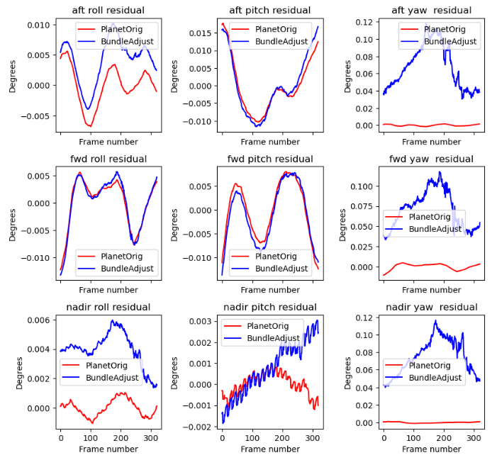
Fig. 8.23 The roll, pitch, and yaw of the camera orientations before and after bundle adjustment for the Aft, Forward, and Nadir cameras (for the center sensor of the Skysat triplet). Plotted with orbit_plot.py (Section 16.45). The best linear fit of this data before bundle adjustment was subtracted to emphasize the differences, which are very small. The cameras centers were tightly constrained here with a large camera position weight. Yet, see Fig. 8.24 for the effect on the reprojection errors.

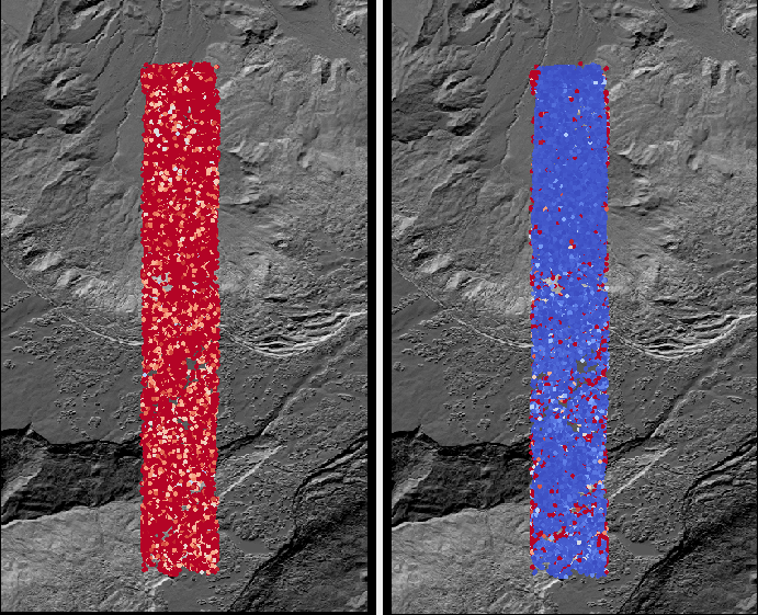
Fig. 8.24 The colorized bundle adjustment camera reprojection errors (pointmap.csv) overlaid on top of the Copernicus 30 m DEM for Grand Mesa, Colorado, before optimization (left) and after (right). Plotted with stereo_gui. Maximum shade of red is reprojection error of at least 5 pixels. The same set of clean interest points was used in both plots. It can be seen that while bundle adjustment changes the cameras very little, it makes a very big difference in how consistent the cameras become.

The camera positions and orientations (the latter in NED coordinates) are summarized in two report files, before and after optimization (Section 16.5.11.9). It is suggested to examine if these are plausible. It is expected that the spacecraft position and orientation will change in a slow and smooth manner, and that these will not change drastically during bundle adjustment.

If desired to do further experiments in bundle adjustment, the existing interest matches can be reused via the options --clean-match-files-prefix and --match-files-prefix. The matches can be inspected with stereo_gui (Section 16.70.9.2).

8.22.1.3. DEM creation

How to decide which pairs of images to choose for stereo and how to combine the resulting DEMs taking into account the stereo convergence angle is described in Section 9.3.5.

8.22.2. Video data

The rest of this section will be concerned with the Video product, which is a set of images recorded together in quick sequence. This is a very capricious dataset, so some patience will be needed to work with it. That is due to the following factors:

• The baseline can be small, so the perspective of the left and right image can be too similar.

• The footprint on the ground is small, on the order of 2 km.

• The terrain can be very steep.

• The known longitude-latitude corners of each image have only a few digits of precision, which can result in poor initial estimated cameras.

Below a recipe for how to deal with this data is described, together with things to watch for and advice when things don’t work.

See also how the Stereo product was processed (Section 8.22.1). That section is newer, and that product was explored in more detail. Stereo products are better-behaved than Video products, so it is suggested to work with Stereo data, if possible, or at least cross-reference with that section the logic below.

8.22.3. The input data

We will use as an illustration a mountainous terrain close to Breckenridge, Colorado. The dataset we fetched is called s4_20181107T175036Z_video.zip. We chose to work with the following four images from it:

1225648254.44006968_sc00004_c1_PAN.tiff
1225648269.40892076_sc00004_c1_PAN.tiff
1225648284.37777185_sc00004_c1_PAN.tiff
1225648299.37995577_sc00004_c1_PAN.tiff

A sample picture from this image set is shown in Fig. 8.25.

It is very important to pick images that have sufficient difference in perspective, but which are still reasonably similar, as otherwise the procedure outlined in this section will fail.

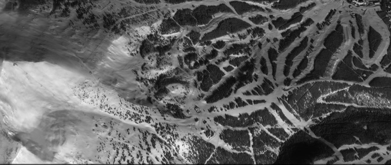
Fig. 8.25 An image used in the SkySat example. Reproduced with permission.

8.22.4. Initial camera models and a reference DEM

Based on vendor’s documentation, these images are \(2560 \times 1080\) pixels. We use the geometric center of the image as the optical center, which turned out to be a reasonable enough assumption (verified by allowing it to float later). Since the focal length is given as 3.6 m and the pixel pitch is \(6.5 \times 10^{-6}\) m, the focal length in pixels is

\[3.6/6.5 \times 10^{-6} = 553846.153846.\]

Next, a reference DEM needs to be found. Recently we recommend getting a Copernicus 30 m DEM (Section 6.1.7.1).

It is very important to note that SRTM DEMs can be relative to the WGS84 ellipsoidal vertical datum, or relative to the EGM96 geoid. In the latter case, dem_geoid (Section 16.19) needs to be used to first convert it to be relative to WGS84. This may apply up to 100 meters of vertical adjustment. See Section 6.1.7.2.

It is good to be a bit generous when selecting the extent of the reference DEM. We will rename the downloaded DEM to ref_dem.tif.

Using the cam_gen tool (Section 16.8) bundled with ASP, we create an initial camera model and a GCP file (Section 16.5.9) for the first image as as follows:

cam_gen 1225648254.44006968_sc00004_c1_PAN.tiff \
  --frame-index output/video/frame_index.csv    \
  --reference-dem ref_dem.tif                   \
  --focal-length 553846.153846                  \
  --optical-center 1280 540                     \
  --pixel-pitch 1 --height-above-datum 4000     \
  --refine-camera                               \
  --gcp-std 1                                   \
  --gcp-file v1.gcp                             \
  -o v1.tsai

This tool works by reading the longitude and latitude of each image corner on the ground from the file frame_index.csv, and finding the position and orientation of the camera that best fits this data. The camera is written to v1.tsai. A GCP file is written to v1.gcp. This will help later with bundle adjustment.

If an input camera exists, such as embedded in the image file, it is strongly suggested to pass it to this tool using the --input-camera option, as it will improve the accuracy of produced cameras (Section 8.22.12).

In the above command, the optical center and focal length are as mentioned earlier. The reference SRTM DEM is used to infer the height above datum for each image corner based on its longitude and latitude. The height value specified via --height-above-datum is used as a fallback option, if for example, the DEM is incomplete, and is not strictly necessary for this example. This tool also accepts the longitude and latitude of the corners as an option, via --lon-lat-values.

The flag --refine-camera makes cam_gen solve a least square problem to refine the output camera. In some cases it can get the refinement wrong, so it is suggested experimenting with and without using this option.

For simplicity of notation, we will create a symbolic link from this image to the shorter name v1.tif, and the GCP file needs to be edited to reflect this. The same will apply to the other files. We will have then four images, v1.tif, v2.tif, v3.tif, v4.tif, and corresponding camera and GCP files.

A good sanity check is to visualize the computed cameras. ASP’s sfm_view tool can be used (Section 16.66). Alternatively, ASP’s orbitviz program (Section 16.46) can create KML files that can then be opened in Google Earth.

We very strongly recommend inspecting the camera positions and orientations, since this may catch inaccurate cameras which will cause problems later.

Another important check is to mapproject these images using the cameras and overlay them in stereo_gui on top of the reference DEM. Here is an example for the first image:

mapproject --t_srs \
'+proj=stere +lat_0=39.4702 +lon_0=253.908 +k=1 +x_0=0 +y_0=0 +datum=WGS84 +units=m' \
ref_dem.tif v1.tif v1.tsai v1_map.tif

Notice that we used above a longitude and latitude around the area of interest. This will need to be modified for your specific example.

8.22.5. Bundle adjustment

At this stage, the cameras should be about right, but not quite exact. We will take care of this using bundle adjustment. We will invoke this tool twice. In the first call we will make the cameras self-consistent. This may move them somewhat, though the --tri-weight constraint that is used below should help. In the second call we will try to bring the back to the original location.

parallel_bundle_adjust                \
  v[1-4].tif v[1-4].tsai              \
  -t nadirpinhole                     \
  --disable-tri-ip-filter             \
  --skip-rough-homography             \
  --force-reuse-match-files           \
  --ip-inlier-factor 2.0              \
  --ip-uniqueness-threshold 0.8       \
  --ip-per-image 20000                \
  --datum WGS84                       \
  --inline-adjustments                \
  --camera-weight 0                   \
  --tri-weight 0.1                    \
  --robust-threshold 2                \
  --remove-outliers-params '75 3 4 5' \
  --ip-num-ransac-iterations 1000     \
  --num-passes 2                      \
  --auto-overlap-params "ref.tif 15"  \
  --num-iterations 1000               \
  -o ba/run

parallel_bundle_adjust                     \
  -t nadirpinhole                          \
  --datum WGS84                            \
  --force-reuse-match-files                \
  --inline-adjustments                     \
  --num-passes 1 --num-iterations 0        \
  --transform-cameras-using-gcp            \
  v[1-4].tif ba/run-v[1-4].tsai v[1-4].gcp \
  -o ba/run

The --auto-overlap-params option used earlier is useful a very large number of images is present and a preexisting DEM of the area is available, which need not be perfectly aligned with the cameras. It can be used to determine each camera’s footprint, and hence, which cameras overlap. Otherwise, use the --overlap-limit option to control how many subsequent images to match with a given image.

The output optimized cameras will be named ba/run-run-v[1-4].tsai. The reason one has the word “run” repeated is because we ran this tool twice. The intermediate cameras from the first run were called ba/run-v[1-4].tsai.

Here we use --ip-per-image 20000 to create a lot of interest points. This will help with alignment later. It is suggested that the user study all these options and understand what they do. We also used --robust-threshold 10 to force the solver to work the bigger errors. That is necessary since the initial cameras could be pretty inaccurate.

It is very important to examine the residual file named:

ba/run-final_residuals_pointmap.csv

(Section 16.5.11.5).

Here, the third column are the heights of triangulated interest points, while the fourth column are the reprojection errors. Normally these errors should be a fraction of a pixel, as otherwise the solution did not converge. The last entries in this file correspond to the GCP, and those should be looked at carefully as well. The reprojection errors for GCP should be on the order of tens of pixels because the longitude and latitude of each GCP are not well-known. This can be done with Section 16.70, which will also colorize the residuals (Section 16.70.6).

It is also very important to examine the obtained match files in the output directory. For that, use stereo_gui with the option --pairwise-matches (Section 16.70.9). If there are too few matches, particularly among very similar images, one may need to increase the value of --epipolar-threshold (or of --ip-inlier-factor for the not-recommended pinhole session). Note that a large value here may allow more outliers, but those should normally by filtered out by bundle_adjust.

Another thing one should keep an eye on is the height above datum of the camera centers as printed by bundle adjustment towards the end. Any large difference in camera heights (say more than a few km) could be a symptom of some failure.

Also look at how much the triangulated points and camera centers moved as a result of bundle adjustment. Appropriate constraints may need to be applied (Section 16.5.6).

Note that using the nadirpinhole session is equivalent to using pinhole and setting --datum.

8.22.6. Creating terrain models

The next steps are to run parallel_stereo and create DEMs.

We will run the following command for each pair of images. Note that we reuse the filtered match points created by bundle adjustment, with the --clean-match-files-prefix option.

i=1
((j=i+1))
st=stereo_v${i}${j}
rm -rfv $st
mkdir -p $st
parallel_stereo --skip-rough-homography       \
  -t nadirpinhole --stereo-algorithm asp_mgm  \
  v${i}.tif v${j}.tif                         \
  ba/run-run-v${i}.tsai ba/run-run-v${j}.tsai \
  --clean-match-files-prefix ba/run           \
  $st/run
point2dem --auto-proj-center \
  --tr 4 --errorimage $st/run-PC.tif

(Repeat this for other values of \(i\).)

See Section 6 for a discussion about various speed-vs-quality choices. See Section 16.57.1 about DEM projection determination.

It is important to examine the mean triangulation error (Section 14.6.1) for each DEM:

gdalinfo -stats stereo_v12/run-IntersectionErr.tif | grep Mean

which should hopefully be no more than 0.5 meters, otherwise likely bundle adjustment failed. One should also compare the DEMs among themselves:

geodiff --absolute stereo_v12/run-DEM.tif stereo_v23/run-DEM.tif -o tmp
gdalinfo -stats tmp-diff.tif | grep Mean

(And so on for any other pair.) Here the mean error should be on the order of 2 meters, or hopefully less.

8.22.7. Mosaicking and alignment

If more than one image pair was used, the obtained DEMs can be mosaicked with dem_mosaic (Section 16.20):

dem_mosaic stereo_v12/run-DEM.tif stereo_v23/run-DEM.tif \
  stereo_v34/run-DEM.tif -o mosaic.tif

This DEM can be hillshaded and overlaid on top of the reference DEM.

The next step is aligning it to the reference.

pc_align --max-displacement 1000 --save-transformed-source-points \
  --alignment-method similarity-point-to-point                    \
  ref_dem.tif mosaic.tif -o align/run

It is important to look at the errors printed by this tool before and after alignment, as well as details about the alignment that was applied. The obtained aligned cloud can be made into a DEM again:

point2dem            \
  --auto-proj-center \
  --tr 4             \
  align/run-trans_source.tif

The absolute difference before and after alignment can be found as follows:

geodiff --absolute mosaic.tif ref_dem.tif -o tmp
gdalinfo -stats tmp-diff.tif | grep Mean

geodiff --absolute  align/run-trans_source-DEM.tif ref_dem.tif -o tmp
gdalinfo -stats tmp-diff.tif | grep Mean

In this case the mean error after alignment was about 6.5 m, which is not too bad given that the reference DEM resolution is about 30 m/pixel.

8.22.8. Alignment of cameras

The transform computed with pc_align can be used to bring the cameras in alignment to the reference DEM. That can be done as follows:

parallel_bundle_adjust -t nadirpinhole --datum wgs84     \
  --force-reuse-match-files                              \
  --inline-adjustments                                   \
  --initial-transform align/run-transform.txt            \
  --apply-initial-transform-only                         \
  v[1-4].tif ba/run-run-v[1-4].tsai -o ba/run

creating the aligned cameras ba/run-run-run-v[1-4].tsai. If pc_align was called with the reference DEM being the second cloud, one should use above the file:

align/run-inverse-transform.txt

as the initial transform.

8.22.9. Mapprojection

If the steep topography prevents good DEMs from being created, one can mapproject the images first onto the reference DEM:

for i in 1 2 3 4; do
  mapproject --tr gridSize ref_dem.tif v${i}.tif \
    ba/run-run-run-v${i}.tsai v${i}_map.tif
done

It is very important to use the same resolution (option --tr) for both images when mapprojecting. That helps making the resulting images more similar and reduces the processing time (Section 6.1.7.4).

Then run parallel_stereo with the mapprojected images, such as:

i=1
((j=i+1))
rm -rfv stereo_map_v${i}${j}
parallel_stereo v${i}_map.tif v${j}_map.tif                   \
  ba/run-run-run-v${i}.tsai ba/run-run-run-v${j}.tsai         \
  --session-type pinhole --alignment-method none              \
  --cost-mode 4 --stereo-algorithm asp_mgm --corr-seed-mode 1 \
  stereo_map_v${i}${j}/run ref_dem.tif

point2dem --auto-proj-center \
  --tr 4 --errorimage        \
  stereo_map_v${i}${j}/run-PC.tif

It is important to note that here we used the cameras that were aligned with the reference DEM. We could have as well mapprojected onto a lower-resolution version of the mosaicked and aligned DEM with its holes filled.

8.22.10. When things fail

Processing SkySat images is difficult, for various reasons mentioned earlier. A few suggestions were also offered along the way when things go wrong.

Problems are usually due to cameras being initialized inaccurately by cam_gen or bundle adjustment not optimizing them well. The simplest solution is often to just try a different pair of images from the sequence, say from earlier or later in the flight, or a pair with less overlap, or with more time elapsed between the two acquisitions. Modifying various parameters may help as well.

We have experimented sufficiently with various SkySat datasets to be sure that the intrinsics (focal length, optical center, and pixel pitch) are usually not the issue, rather the positions and orientations of the cameras.

8.22.11. Structure from motion

In case cam_gen does not create sufficiently good cameras, one can attempt to use the camera_solve tool (Section 9). This will create hopefully good cameras but in an arbitrary coordinate system. Then we will transfer those to the world coordinates using GCP.

Here is an example for two cameras:

out=out_v12
ba_params="--num-passes 1 --num-iterations 0
   --transform-cameras-using-gcp"
theia_overdides="--sift_num_levels=6 --lowes_ratio=0.9
  --min_num_inliers_for_valid_match=10
  --min_num_absolute_pose_inliers=10
  --bundle_adjustment_robust_loss_function=CAUCHY
  --post_rotation_filtering_degrees=180.0 --v=2
  --max_sampson_error_for_verified_match=100.0
  --max_reprojection_error_pixels=100.0
  --triangulation_reprojection_error_pixels=100.0
  --min_num_inliers_for_valid_match=10
  --min_num_absolute_pose_inliers=10"
rm -rfv $out
camera_solve $out --datum WGS84 --calib-file v1.tsai  \
    --bundle-adjust-params "$ba_params v1.gcp v2.gcp" \
    v1.tif v2.tif

The obtained cameras should be bundle-adjusted as done for the outputs of cam_gen. Note that this tool is capricious and its outputs can be often wrong. In the future it will be replaced by something more robust.

8.22.12. RPC models

Some SkySat datasets come with RPC camera models, typically embedded in the images. This can be verified by running:

gdalinfo -stats output/video/frames/1225648254.44006968_sc00004_c1_PAN.tiff

We found that these models are not sufficiently robust for stereo. But they can be used to create initial guess pinhole cameras (Section 20.1) with cam_gen.

We will use the RPC camera model instead of longitude and latitude of image corners to infer the pinhole camera position and orientation. This greatly improves the accuracy and reliability.

Here is an example:

img=output/video/frames/1225648254.44006968_sc00004_c1_PAN.tiff
cam_gen $img --reference-dem ref_dem.tif --focal-length 553846.153846  \
   --optical-center 1280 540 --pixel-pitch 1 --height-above-datum 4000 \
   --refine-camera --gcp-std 1 --input-camera $img                     \
   -o v1_rpc.tsai --gcp-file v1_rpc.gcp

Note that the Breckenridge dataset does not have RPC data, but other datasets do. If the input camera is stored separately in a camera file, use that one with --input-camera.

If an RPC model is embedded in the image, one can validate how well the new Pinhole camera approximates the existing RPC camera with cam_test (Section 16.9), with a command like:

cam_test --image image.tif --cam1 image.tif --cam2 out_cam.tsai \
    --height-above-datum 4000

Then one can proceed as earlier (particularly the GCP file can be edited to reflect the shorter image name).

One can also regenerate the provided SkySat RPC model as:

cam2rpc -t rpc --dem-file dem.tif input.tif output.xml

Here, the reference DEM should go beyond the extent of the image. This tool makes it possible to decide how finely to sample the DEM, and one can simply use longitude-latitude and height ranges instead of the DEM.

We assumed in the last command that the input image implicitly stores the RPC camera model, as is the case for SkySat.

Also, any pinhole camera models obtained using our software can be converted to RPC models as follows:

cam2rpc --dem-file dem.tif input.tif input.tsai output.xml

8.22.13. Bundle adjustment using reference terrain

At this stage, if desired, but this is rather unnecessary, one can do joint optimization of the cameras using dense and uniformly distributed interest points, and using the reference DEM as a constraint. This should make the DEMs more consistent among themselves and closer to the reference DEM.

It is also possible to float the intrinsics, per Section 12.2.1, which sometimes can improve the results further.

For that, one should repeat the stereo_tri part of of the stereo commands from Section 8.22.6 with the flags --num-matches-from-disp-triplets 10000 and --unalign-disparity to obtain dense interest points and unaligned disparity. (To not generate the triangulated point cloud after this, add the option --compute-point-cloud-center-only.) Use --num-matches-from-disparity 10000 if the images are large, as the earlier related option can be very slow then.

The match points can be examined as:

stereo_gui v1.tif v2.tif stereo_v12/run-disp-v1__v2.match

and the same for the other image pairs. Hopefully they will fill as much of the images as possible. One should also study the unaligned disparities, for example:

stereo_v12/run-v1__v2-unaligned-D.tif

by invoking disparitydebug on it and then visualizing the two obtained images. Hopefully these disparities are dense and with few holes.

The dense interest points should be copied to the new bundle adjustment directory, such as:

mkdir -p ba_ref_terrain
cp stereo_v12/run-disp-v1__v2.match ba_ref_terrain/run-v1__v2.match

and the same for the other ones (note the convention for match files in the new directory). The unaligned disparities can be used from where they are.

Then bundle adjustment using the reference terrain constraint proceeds as follows:

disp_list=$(ls stereo_v[1-4][1-4]/*-unaligned-D.tif)
bundle_adjust v[1-4].tif  ba/run-run-run-v[1-4].tsai -o ba_ref_terrain/run    \
--reference-terrain ref_dem.tif --disparity-list "$disp_list"                 \
--max-num-reference-points 10000000 --reference-terrain-weight 50             \
--parameter-tolerance 1e-12 -t nadirpinhole --max-iterations 500              \
--overlap-limit 1 --inline-adjustments --robust-threshold 2                   \
--force-reuse-match-files --max-disp-error 100 --camera-weight 0

If invoking this creates new match files, it means that the dense match files were not copied successfully to the new location. If this optimization is slow, perhaps too many reference terrain points were picked.

This will create, as before, the residual file named:

ba_ref_terrain/run-final_residuals_pointmap.csv

showing how consistent are the cameras among themselves, and in addition, a file named:

ba_ref_terrain/run-final_residuals_reference_terrain.txt

which tells how well the cameras are aligned to the reference terrain. The errors in the first file should be under 1 pixel, and in the second one should be mostly under 2-3 pixels (both are the fourth column in these files).

The value of --reference-terrain-weight can be increased to make the alignment to the reference terrain a little tighter.

It is hoped that after running parallel_stereo with these refined cameras, the obtained DEMs will differ by less than 2 m among themselves, and by less than 4 m as compared to the reference DEM.

8.22.14. Floating the camera intrinsics

If desired to float the focal length as part of the optimization, one should pass in addition, the options:

--solve-intrinsics --intrinsics-to-float 'focal_length'

Floating the optical center can be done by adding it in as well.

It is important to note that for SkySat the intrinsics seem to be already quite good, and floating them is not necessary and is only shown for completeness. If one wants to float them, one should vary the focal length while keeping the optical center fixed, and vice versa, and compare the results. Then, with the result that shows most promise, one should vary the other parameter. If optimizing the intrinsics too aggressively, it is not clear if they will still deliver better results with other images or if comparing with a different reference terrain.

Yet, if desired, one can float even the distortion parameters. For that, the input camera files need to be converted to some camera model having these (see Section 20.1), and their values can be set to something very small. One can use the Brown-Conrady model, for example, so each camera file must have instead of NULL at the end the fields:

BrownConrady
xp  = -1e-12
yp  = -1e-12
k1  = -1e-10
k2  = -1e-14
k3  = -1e-22
p1  = -1e-12
p2  = -1e-12
phi = -1e-12

There is always a chance when solving these parameters that the obtained solution is not optimal. Hence, one can also try using as initial guesses different values, for example, by negating the above numbers.

One can also try to experiment with the option --heights-from-dem, and also with --robust-threshold if it appears that the large errors are not minimized enough.