8.15. Chandrayaan-2 lunar orbiter

The example here shows how to create a 3D terrain model with Chandrayaan-2 lunar orbiter data, using both the Orbiter High Resolution Camera (OHRC) and the Terrain Mapping Camera-2 (TMC-2).

This workflow needs ASP 3.7.0 or later, installed via conda together with its bundled ISIS, ALE, and USGSCSM, as described in the environment setup below.

Chandrayaan-2 ISIS data should be downloaded as documented further down.

8.15.1. Environment setup

Install ASP 3.7.0 as documented in Section 2.2. That release ships its own custom-built ISIS 10.0.0, along with custom ALE, USGSCSM, and SpiceQL, with the Chandrayaan-2 camera fixes already included. These are newer than the current public ISIS, ALE, and USGSCSM releases, and are needed for the fore and aft TMC-2 cameras. The conda environment (named asp there) already contains all of them. Activate it and point ISIS at it:

conda activate asp
export ISISROOT=$CONDA_PREFIX

Set the location of the ISIS data area (to be downloaded next):

export ISISDATA=$HOME/projects/isisdata
export ALESPICEROOT=$ISISDATA

The kernel download below uses rclone. If it is not already in the environment, install it with conda install -c conda-forge rclone.

See also the USGS ISIS TMC documentation.

8.15.2. ISIS kernels download

The mission kernels are fetched with downloadIsisData, which is shipped with ISIS:

downloadIsisData chandrayaan2 $ISISDATA

Note that the full chandrayaan2 directory is large (about 200 GB), of which essentially all is reconstructed attitude kernels (ck) covering the entire mission since 2019. For a single OHRC image only one or two ck files are needed. Fetching everything except ck takes only a few hundred MB:

downloadIsisData chandrayaan2 $ISISDATA --exclude="kernels/ck/**"

The command:

rclone --config $ISISROOT/etc/isis/rclone.conf \
  ls chandrayaan2:kernels/ck/

lists all available ck files. This can help pick the ones that span the acquisition time of the products to be processed.

The ck files matching the orbit dates of interest can then be fetched individually with rclone, such as:

rclone                                          \
  --config $ISISROOT/etc/isis/rclone.conf       \
  copy                                          \
  chandrayaan2:kernels/ck/                      \
  $ISISDATA/chandrayaan2/kernels/ck/            \
  --include="ch2_att_27Jul2020_04Sep2020_v1.bc" \
  --include="ch2_att_27Aug2020_04Oct2020_v1.bc" \
  --no-traverse -P

8.15.3. Fetching images

Images, orthoimages, and DEMs for the OHRC and TMC-2 cameras can be downloaded from ISRO.

Each download is a zip. After unzipping, locate the .img and .xml files and move them into a working directory. Keep the original ISRO filenames; a rename can break isisimport.

8.15.4. Orbiter High Resolution Camera

The OHRC instrument is a high-resolution camera with a 0.25 m ground sample distance (GSD). It can adjust its look angle and acquire stereo pairs (Section 8.1).

8.15.4.1. Input data

Download the OHRC stereo pair from ISRO as described in Section 8.15.3. We selected the region of interest to be between 20 and 21 degrees in longitude, and -70 to -67 degrees in latitude. The prefixes are:

ch2_ohr_nrp_20200827T0030107497_d_img_d18
ch2_ohr_nrp_20200827T0226453039_d_img_d18

We also got a TMC-2 orthoimage and corresponding DEM with the prefixes:

ch2_tmc_ndn_20231101T0125121377_d_oth_d18
ch2_tmc_ndn_20231101T0125121377_d_dtm_d18

These are at lower resolution but useful for context.

Fig. 8.26 From left to right: The first and second OHRC images, and their approximate extent in the (many times larger) TMC-2 ortho image. Note that the illumination in the TMC-2 ortho image is very different.

8.15.4.2. Preprocessing

The steps below assume the ASP 3.7.0 conda environment, which ships a custom build of ISIS, ALE, and USGSCSM (Section 2.2). If spiceinit or isd_generate -k errors, the active ISIS, ALE, or USGSCSM is likely too old, or a separately installed ISIS is being used instead of the one bundled with ASP. Activate the ASP 3.7.0 environment, or use a recent development ISIS build from 2026.06.07 or later from the dev label of the usgs-astrogeology channel (usgs-astrogeology/label/dev).

Each calibrated image dataset has .img and .xml files, with raw data and a PDS-4 label.

The isisimport command converts the raw image to a .cub file:

isisimport                                             \
  from = ch2_ohr_nrp_20200827T0030107497_d_img_d18.xml \
  to   = ch2_ohr_nrp_20200827T0030107497_d_img_d18.cub

(and same for the second image). The PDS4 template is auto-detected in ISIS 10.

For simplicity, the output cub files are renamed to ohrc/img1.cub and ohrc/img2.cub.

The isisimport command only works with raw images and not with ortho images.

The SPICE kernels are attached with spiceinit:

spiceinit from = ohrc/img1.cub

This expects the SPICE kernels for Chandrayaan-2 to exist locally under $ISISDATA/chandrayaan2/ (see the download instructions above). For more information on ISIS data, see Section 2.3.1 and the links from there.

Next, CSM cameras are created with isd_generate from the ALE package, following the linescan recipe in Section 8.12.2.1:

export ALESPICEROOT=$ISISDATA
isd_generate -k ohrc/img1.cub ohrc/img1.cub
isd_generate -k ohrc/img2.cub ohrc/img2.cub

It is expected that the environment is activated with conda activate, with ISISROOT set to $CONDA_PREFIX, and $ISISDATA and $ALESPICEROOT set, as described in the environment setup section above (not just the environment’s bin directory added to the path). Chandrayaan-2 uses the SpiceQL mission database, and skipping conda activate can make isd_generate crash instead of printing a clear error, as SpiceQL then cannot find its configuration under $CONDA_PREFIX.

Check each produced CSM camera file with cam_test (Section 16.9), against itself and against the .cub camera, before proceeding.

The images can be inspected with stereo_gui (Section 16.73), as:

stereo_gui ohrc/img1.cub ohrc/img2.cub

The resulting cub files are very large, on the order of 12,000 x 101,075 pixels. The full images are processed throughout.

8.15.4.3. Bundle adjustment

We found that these images have notable pointing error, so bundle adjustment (Section 16.5) is needed:

bundle_adjust                           \
  ohrc/img1.cub ohrc/img2.cub           \
  ohrc/img1.json ohrc/img2.json         \
  --num-iterations 100 --num-passes 2   \
  --camera-weight 0 --tri-weight 0.1    \
  --remove-outliers-params "75 3 50 50" \
  --ip-per-image 50000                  \
  --max-pairwise-matches 50000          \
  -o ba/run

This stereo pair has a convergence angle of about 25 degrees (Section 16.5.11.4). Inspect the report files (Section 16.5.11); the reprojection error should be sub-pixel.

Fig. 8.27 The left and right OHRC images, and the clean interest point matches between them. These can be plotted with stereo_gui, Section 16.73.9).

8.15.4.4. Stereo

A first DEM is made from the raw images with local epipolar alignment (Section 17.1.2) and the bundle-adjusted cameras. This is the same approach used for the TMC triplet (Section 8.15.5.6). This method does not require the cameras to be correctly registered to the ground.

This needs build 2026/08/21 (Section 2.1) or later, which improved the robustness of local-epipolar alignment.

parallel_stereo                     \
  --alignment-method local_epipolar \
  --stereo-algorithm asp_mgm        \
  --subpixel-mode 9                 \
  --ip-per-tile 300                 \
  --nodes-list nodes.txt            \
  ohrc/img1.cub ohrc/img2.cub       \
  ba/run-img1.adjusted_state.json   \
  ba/run-img2.adjusted_state.json   \
  stereo/run

A generous --ip-per-tile gives the per-tile local alignment enough interest points on these long, narrow strips, so few tiles are left unmatched.

See Section 8.22 for running on multiple nodes. See Section 6 for the various correlation and subpixel algorithms available.

Make the DEM at 1 m (4x image resolution), with the orthoimage and triangulation error (Section 16.57):

point2dem --tr 1.0 --errorimage --orthoimage \
  stereo/run-PC.tif stereo/run-L.tif

The resulting files are named stereo/run-DEM.tif, stereo/run-DRG.tif, and stereo/run-IntersectionErr.tif.

The deep-shadow crater on this strip has almost no image signal, so stereo leaves an artifact there: a spurious block in the DEM with high triangulation error. Mask it out with the orthoimage, which is near zero in shadow. First build a binary mask that is 1 on lit terrain and 0 in shadow (Section 16.34.1.3):

thresh=0.1
image_calc -c "gte(var_0, $thresh, 1, 0)" \
  --output-nodata-value -1e+6             \
  -d float32                              \
  stereo/run-DRG.tif                      \
  -o stereo/run-shadow_mask.tif

Choose the threshold from the orthoimage histogram, large enough to remove the black crater but not the lit terrain (here 0.1). Then apply the mask to the DEM, the orthoimage, and the triangulation error, which share the same grid (Section 16.34.1.2):

image_calc -c "eq(var_1, 0, -9999, var_0)"      \
  --output-nodata-value -9999                   \
  -d float32                                    \
  stereo/run-DEM.tif stereo/run-shadow_mask.tif \
  -o stereo/run-DEM_masked.tif

The same command is applied to run-DRG.tif and run-IntersectionErr.tif. The masked products are used for all inspection and figures below.

8.15.4.5. Reference DEM

A reference DEM is needed for alignment and mapprojection. Here the choice is a Kaguya TC DTM (~32 m/pixel, Section 8.14.5), which is finer than the wider-area LOLA gridded DEMs. The site is around -68 degrees latitude, within Kaguya’s reach. For the TMC dataset, closer to the pole where Kaguya does not reach (as of 2026-08, though this may change), the polar LOLA product was the better choice (Section 8.15.5.4).

Merge the Kaguya tiles that cover the site into one DEM with dem_mosaic (Section 16.20), and call it ref.tif.

Choose a local projection, centered on the site, that is used for all steps below. Here we use a south polar stereographic projection:

proj="+proj=stere +lat_0=-68.4 +lon_0=20.9 +k=1 +x_0=0 +y_0=0 +R=1737400 +units=m +no_defs"

Convert the reference to this projection if it is not already in it (Section 16.25):

gdalwarp -r cubicspline -t_srs "$proj" kaguya_merged.tif ref.tif

A Kaguya DTM can have holes. Fill them (Section 16.20.2.9) and optionally blur the result (dem_mosaic --dem-blur-sigma 5, Section 16.20.2.6), so the DEM used for mapprojection is gap-free.

8.15.4.6. Alignment to a reference DEM

The cameras must be aligned to the reference DEM’s coordinate system. The OHRC DEM is shifted from the reference by about 2.1 km along the track. DEM alignment is not fully robust, and the best method depends on the data, so it is worth trying more than one (Section 16.54). The robust route here is correlation-based alignment (Section 16.54.3.5): a bounded dense correlation cannot slide globally the way ICP can. It is automated but can be fragile, so inspect the result. Also see the analogous section for TMC (Section 8.15.5.7).

Regrid the OHRC DEM and the reference to the same grid, projection, and extent with gdalwarp (Section 16.25):

gdalwarp -r cubicspline -t_srs "$proj" \
  -te <ref extent> -tr 32 32           \
  stereo/run-DEM.tif ohrc_on_ref.tif

Hillshade both (Section 16.29.1):

gdaldem hillshade -multidirectional ref.tif         ref_hill.tif
gdaldem hillshade -multidirectional ohrc_on_ref.tif src_hill.tif

Fig. 8.28 The regridded OHRC DEM and the Kaguya reference, both hillshaded, with a shared projection, grid, and extent. They must look visually similar for the correlation to succeed. The reference goes beyond the OHRC DEM to take into account the initial misregistration.

Correlate the hillshades (Section 16.17) and extract a dense match file. The search range must large enough to incorporate the expected misalignment (shift). Here the shift was found visually to be about 66 px (2.1 km at 32 m), so --corr-search -100 -100 100 100 is enough. For a larger shift, increase this range. Too large a search range results in slow processing and risks locking onto a wrong solution.

parallel_stereo --correlator-mode    \
  --stereo-algorithm asp_mgm         \
  --subpixel-mode 9                  \
  --corr-kernel 9 9                  \
  --corr-search -100 -100 100 100    \
  --ip-per-image 40000               \
  --num-matches-from-disparity 40000 \
  ref_hill.tif src_hill.tif run_corr/run

Inspect the disparity run_corr/run-F.tif (Section 16.23.2). A smoothly varying, near-constant shift means a good lock. Inspect this dense match file then pass it to pc_align (Section 16.54.3.5):

pc_align --max-displacement -1 --num-iterations 0         \
  --max-num-reference-points 1000000                      \
  --match-file run_corr/run-disp-ref_hill__src_hill.match \
  --initial-transform-from-hillshading rigid              \
  --initial-transform-ransac-params 1000 3                \
  --save-transformed-source-points                        \
  ref.tif ohrc_on_ref.tif -o run_align/run

Grid the aligned cloud run_align/run-trans_source.tif with point2dem and inspect it against the reference and the DEM before alignment.

8.15.4.7. Mapprojection

The transform run_align/run-transform.txt maps the OHRC DEM to the reference. Apply it to the bundle-adjusted cameras (Section 16.54.14), so both cameras move into the reference frame:

bundle_adjust                                     \
  ohrc/img1.cub ohrc/img2.cub                     \
  ba/run-img1.adjusted_state.json                 \
  ba/run-img2.adjusted_state.json                 \
  --initial-transform run_align/run-transform.txt \
  --apply-initial-transform-only                  \
  --inline-adjustments                            \
  -o ba_align/run

Mapproject each image at the native ~0.25 m/pixel resolution onto the reference DEM, with the aligned cameras. The reference is gap-free, so no hole filling is needed. The command for the first image is below; the second is identical with its own cub and camera:

mapproject --tr 0.25                     \
  --t_srs "$proj"                        \
  ref.tif                                \
  ohrc/img1.cub                          \
  ba_align/run-img1.adjusted_state.json  \
  ohrc/img1.map.tif

The projection variable was set earlier in the text. Both mapprojected images inherit the reference DEM’s projection, so they are on a common grid.

8.15.4.8. Stereo with mapprojected images

Run stereo with mapprojected images (Section 6.1.7) and the aligned CSM cameras:

parallel_stereo                         \
  --alignment-method none               \
  --stereo-algorithm asp_mgm            \
  --subpixel-mode 9                     \
  --nodes-list nodes.txt                \
  ohrc/img1.map.tif ohrc/img2.map.tif   \
  ba_align/run-img1.adjusted_state.json \
  ba_align/run-img2.adjusted_state.json \
  stereo_map/run                        \
  ref.tif

Produce the DEM at 1 m per pixel, with the orthoimage and triangulation error:

point2dem --tr 1.0      \
  --t_srs "$proj"       \
  --errorimage          \
  --orthoimage          \
  stereo_map/run-PC.tif \
  stereo_map/run-L.tif

As in the local-epipolar pass, the deep-shadow crater is a data void. Apply the same shadow mask (described above) to the DEM, orthoimage, and triangulation error before inspecting.

Fig. 8.29 The final DEM (hillshade), orthoimage, and triangulation error (0 to 0.5 m), after masking the shadow crater. The median triangulation error is 0.07 m. The horizontal striping in the error is along-track jitter at the 0.25 m GSD scale, which could be reduced by solving for jitter (Section 16.39).

This is a solid ~65.6 km^2 strip, improving on the first pass in both coverage (65.6 vs 64.2 km^2) and triangulation error (0.070 vs 0.082 m).

8.15.4.9. Vertical accuracy vs LOLA

The reference itself may be slightly offset from LOLA (Section 19.12.3), the global standard, and the DEM inherits that. Difference the created aligned DEM and the reference against the raw LOLA shots (Section 19.12.3, Section 16.26) to check:

geodiff stereo_map/run-DEM_masked.tif lola_shots.csv \
  --csv-format "2:lon 3:lat 4:radius_km" -o dem_vs_lola

Fig. 8.30 Final DEM minus Kaguya (raster), and the DEM and Kaguya each minus the LOLA shots, all cropped to the DEM extent and clamped +-10 m. The masked crater is the empty hole. The DEM is essentially unbiased against Kaguya (median -0.02 m) and sub-meter against the raw LOLA shots (-0.47 m). Kaguya itself sits about -0.60 m below LOLA over this area, so the DEM matches true ground about as well as the reference it aligned to; the small residual is that reference offset, not a stereo error.

8.15.4.10. Refinement of alignment to LOLA

The DEM is now within about a meter of LOLA, the global standard. Since it is already in the ballpark, the alignment can be refined directly against the LOLA shots with ordinary point-to-plane ICP (Section 16.54.3), which now converges. Pass the DEM first, as the denser cloud (Section 16.54):

pc_align --max-displacement 250                \
  --csv-format "2:lon 3:lat 4:radius_km"       \
  --save-inv-transformed-reference-points      \
  stereo_map/run-DEM_masked.tif lola_shots.csv \
  -o align_lola/run

Here the DEM is the reference (the denser cloud), so the roles are reversed and the inverse transform maps it onto LOLA. The produced cloud align_lola/run-trans_reference.tif is that DEM in the LOLA frame; grid it with point2dem (Section 16.57) as before. That same inverse transform (Section 16.54.6) can also be applied to the cameras (Section 16.54.14).

The correction is small but real: a north-east-down translation of about (2.6, 1.8, 0.5) meters, with a very small rotation. It is mostly a 3 m horizontal nudge plus a 0.5 m down shift that removes the slight vertical bias (the DEM minus the LOLA shots goes from a median of -0.47 m to about 0) and tightens the fit by roughly 20 percent (NMAD from 1.74 to 1.39 m).

8.15.5. Terrain Mapping Camera-2

The TMC-2 instrument is a 3-line pushbroom camera, with separate forward (fwd), downward-pointing (nadir), and backward (aft) detectors, The look angles differ by about 25 degrees, which is well-suited to stereo. The ground sample distance is about 5 meters at 100 km altitude.

All three detectors record simultaneously, so a substantial ground swath is imaged by all of them.

8.15.5.1. Input data

Download the TMC-2 forward, nadir, and aft stereo triplet from ISRO as described in Section 8.15.3. The three acquisitions cover a shared ground swath on the same orbit pass:

ch2_tmc_ncf_20231101T0125121344_d_img_d18
ch2_tmc_ncn_20231101T0125121377_d_img_d18
ch2_tmc_nca_20231101T0125121377_d_img_d18

Each detector image is about 4000 by 190000 pixels. In this example the site is near the lunar south pole, and the track runs from about -60 to -89 degrees latitude. We process the full track (not a crop) and use all three looks, forming two stereo pairs: fwd-nadir and nadir-aft.

Fig. 8.31 The three raw TMC-2 looks (forward, nadir, aft), before any mapprojection. These are long and narrow push-broom images. Deeply shadowed terrain is recorded with a pixel value of 0 which is also the nodata value.

8.15.5.2. Preprocessing

These steps require the ASP 3.7.0 conda environment, which ships a custom build of ISIS, ALE, and USGSCSM (Section 2.2).

All three TMC-2 detectors are processed the same way as OHRC above, using the CSM camera models (Section 8.12). Convert each raw image to a cub:

isisimport                                             \
  from = ch2_tmc_ncf_20231101T0125121344_d_img_d18.xml \
  to   = ch2_tmc_ncf_20231101T0125121344_d_img_d18.cub

and the same for the nadir and aft images. For simplicity, the output cub files are renamed to tmc/fwd.cub, tmc/nadir.cub, and tmc/aft.cub. Then attach the kernels and create the CSM camera for each, using isd_generate with the -k option:

spiceinit from = tmc/fwd.cub
isd_generate -k tmc/fwd.cub tmc/fwd.cub

and the same for tmc/nadir.cub and tmc/aft.cub.

An error here likely means that the active ISIS is not the one bundled with ASP 3.7.0, such as a separately installed public ISIS 10.0.0 or 10.0.0_RC2. Alternatively, install a recent development ISIS build from 2026.06.07 or later from the dev label of the usgs-astrogeology channel (usgs-astrogeology/label/dev).

8.15.5.3. Alternative creation of CSM cameras

With older ISIS, skip spiceinit altogether and follow the steps below.

Create for ALE a metakernel under $ALESPICEROOT (which is usually set to $ISISDATA) to locate the SPICE kernels. That is needed since USGS Chandrayaan-2 ISIS data area does not ship one (as of 2026-08-02). Its path should be:

$ISISDATA/chandrayaan2/kernels/mk/ch2_v01.tm

It lists the kernel files. The values in PATH_VALUES should be absolute, due to limitations in ALE, and correct for the local file system. See the NAIF Metakernel reference for the format, and compare with existing .tm files for other missions. Then run isd_generate without the -k option:

export ALESPICEROOT=$ISISDATA
isd_generate tmc/fwd.cub
isd_generate tmc/aft.cub

Check each JSON with cam_test (Section 16.9).

8.15.5.4. Reference DEM

A reference DEM is needed, for alignment and mapprojection.

Near the lunar south pole, a gridded LOLA polar DEM is the natural choice (Section 11.10.2). The product LDEM_60S_120M covers -60 to -90 degrees at 120 m per pixel in one tile, spanning the full track. A Kaguya TC DTM (~32 m/pixel, Section 8.14.5) is at a finer resolution, but does not reach the pole, and the wider-area LOLA products may be coarser than 120 m away from poles. So LDEM_60S_120M at 120 m is the best available reference here. Call it ref.tif.

Choose a local projection that is then used for all steps below. Here we will go with the south polar stereographic projection:

proj="+proj=stere +lat_0=-90 +lon_0=0 +k=1 +x_0=0 +y_0=0 +R=1737400 +units=m +no_defs"

The reference DEM is already in this projection, otherwise it could be converted to it with a command such as:

gdalwarp -r cubicspline -t_srs "$proj" LDEM_60S_120M.tif ref.tif

Such DEMs can be very large. In that case it is suggested to pass an extent to this command with the -te option.

A LOLA gridded DEM is already gap-free. For a reference DEM with holes (such as a prior TMC or Kaguya DTM), fill them (Section 16.20.2.9) and optionally blur the DEM (dem_mosaic --dem-blur-sigma 5, Section 16.20.2.6) before use.

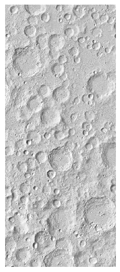
Fig. 8.32 Hillshade of the 120 m LOLA reference DEM, cropped to a region around the area of interest. This is coarse relative to TMC but has the correct absolute geometry, which is needed for alignment and mapprojection.

8.15.5.5. Bundle adjustment

These images have a notable pointing error, so a joint bundle adjustment of the triplet is needed (Section 16.5). The three images (.cub files) and their CSM cameras are passed in the same order:

bundle_adjust                              \
  tmc/fwd.cub tmc/nadir.cub tmc/aft.cub    \
  tmc/fwd.json tmc/nadir.json tmc/aft.json \
  --num-iterations 100 --num-passes 2      \
  --camera-weight 0 --tri-weight 0.1       \
  --remove-outliers-params "75 3 50 50"    \
  --ip-per-tile 400                        \
  --matches-per-tile 200                   \
  --max-pairwise-matches 200000            \
  -o ba/run

Inspect the match files (Section 16.73.9.2), the pixel reprojection errors, and other metrics (Section 16.5.11).

Fig. 8.33 Pixel reprojection errors per triangulated point, in a local projection. The residuals are sub-pixel almost everywhere.

8.15.5.6. Stereo with local epipolar alignment

A first DEM is produced from the raw images and bundle-adjusted cameras with local_epipolar image alignment (Section 17.1.2). This method does not require the cameras to be correctly registered to the ground but only self-consistent.

This requires build 2026/08/21 or later (Section 2.1), incorporating some robustness fixes for this method.

Run each pair such as:

parallel_stereo                       \
  --alignment-method local_epipolar   \
  --stereo-algorithm asp_mgm          \
  --subpixel-mode 9                   \
  --ip-per-tile 300                   \
  --nodes-list nodes.txt              \
  tmc/fwd.cub tmc/nadir.cub           \
  ba/run-fwd.adjusted_state.json      \
  ba/run-nadir.adjusted_state.json    \
  stereo_fn/run

See Section 8.22 for running on multiple nodes. See Section 6 for the various correlation and subpixel algorithms available.

Run point2dem to produce a DEM at 20 m per pixel (about 4x the input GSD, Section 16.57.4), and to create the triangulation error image (Section 16.57.2.2):

point2dem --tr 20      \
  --t_srs "$proj"      \
  --errorimage         \
  stereo_fn/run-PC.tif \
  stereo_fn/run-L.tif

The projection variable was set earlier in the text.

The two pair DEMs are then merged into one with dem_mosaic (Section 16.20):

dem_mosaic stereo_fn/run-DEM.tif stereo_na/run-DEM.tif \
  -o tmc_merged.tif

Fig. 8.34 Left to right: fwd-nadir hillshaded DEM, nadir-aft DEM, fwd-nadir triangulation error (Section 14.6.1), nadir-aft triangulation error. The coverage degrades in shadows. A later plot will have a close-up of a well-lit region.

8.15.5.7. Alignment to LOLA

The cameras must be aligned to the reference DEM’s coordinate system. The merged DEM is shifted from the usual LOLA global reference (here by about 3 km along the track). This is quite large. Aligning to LOLA with the usual ICP point-to-plane method (Section 16.54.3) fails. What worked is to do a coarse alignment first. The best method depends on the data; a narrow swath such as OHRC needs a different one (Section 8.15.4.6).

Coarsen the created merged TMC DEM to the same grid, projection, and extent as ref.tif:

gdalwarp -r average -tr 120 120 -t_srs "$proj" \
  tmc_merged.tif tmc_merged_120m.tif

Overlay this onto ref.tif and inspect both. They should appear similar and with a visible shift.

Here we choose to do a first alignment with sparse matches produced from hillshades (Section 16.54.3.4):

pc_align                                      \
  --initial-transform-from-hillshading rigid  \
  --max-displacement 3000                     \
  --num-iterations 0                          \
  ref.tif tmc_merged_120m.tif                 \
  -o align/seed

If this fails, consider correlation-based alignment (Section 16.54.3.5), with a search range based on the observed shift (Section 14.4.2).

The alignment is refined with point-to-plane ICP, seeded by the first transform:

pc_align                                       \
  --initial-transform align/seed-transform.txt \
  --alignment-method point-to-plane            \
  --max-displacement 300                       \
  --num-iterations 1000                        \
  --save-transformed-source-points             \
  ref.tif tmc_merged_120m.tif                  \
  -o align/run

The output align/run-transform.txt is the combined transform of both calls.

Run point2dem on the transformed source cloud and overlay it on ref.tif for inspection.

Apply that transform to the three cameras, so all of them move into the LOLA frame together (Section 16.54.14):

bundle_adjust                                 \
  tmc/fwd.cub tmc/nadir.cub tmc/aft.cub       \
  ba/run-fwd.adjusted_state.json              \
  ba/run-nadir.adjusted_state.json            \
  ba/run-aft.adjusted_state.json              \
  --initial-transform align/run-transform.txt \
  --apply-initial-transform-only              \
  --inline-adjustments                        \
  -o ba_align/run

8.15.5.8. Mapprojection

Mapproject each cub at the native ~5 m/pixel resolution onto the aligned reference, with the aligned cameras. The command for the forward look is below; the nadir and aft looks are identical with their own cub and camera:

mapproject --tr 5                      \
  --t_srs "$proj"                      \
  ref.tif                              \
  tmc/fwd.cub                          \
  ba_align/run-fwd.adjusted_state.json \
  tmc/fwd.map.tif

The mapprojected images inherit the reference DEM’s projection (the south polar stereographic above), so all three are on a common grid.

Overlay these and the hillshaded reference DEM with georeference information in stereo_gui (Section 16.73) and confirm that they are all in agreement.

Fig. 8.35 The three mapprojected looks (forward, nadir, aft). Areas in shadow are set to no-data and appear black.

8.15.5.9. Stereo with mapprojected images

For each image pair, run stereo with mapprojected images (Section 6.1.7) and the aligned CSM cameras, such as:

parallel_stereo                          \
  --alignment-method none                \
  --stereo-algorithm asp_mgm             \
  --subpixel-mode 9                      \
  --nodes-list nodes.txt                 \
  tmc/fwd.map.tif tmc/nadir.map.tif      \
  ba_align/run-fwd.adjusted_state.json   \
  ba_align/run-nadir.adjusted_state.json \
  stereo_fn_map/run                      \
  ref.tif

Produce DEMs at 20 m per pixel:

point2dem --tr 20 \
  --t_srs "$proj" \
  --errorimage    \
  stereo_fn_map/run-PC.tif

Merge the results as before:

dem_mosaic stereo_fn_map/run-DEM.tif stereo_na_map/run-DEM.tif \
  -o tmc_merged_map.tif

Fig. 8.36 Mapprojected-pass DEMs (hillshaded) and triangulation error (0 to 5 m), left to right: fwd-nadir DEM, nadir-aft DEM, fwd-nadir error, nadir-aft error. The triangulation error is visibly lower than in the local-epipolar pass (medians drop by roughly 10 to 25 percent), which is the payoff of mapprojected stereo.

Fig. 8.37 A close-up DEM after stereo with mapprojection, showing the upper part of the track. The quality is very good on illuminated terrain, with small craters resolved. Results degrade gracefully toward shadowed areas.

8.15.5.10. Evaluation

To validate the results, compare against LOLA. First difference the DEM against the gridded LOLA reference (Section 16.26):

geodiff tmc_merged_map.tif ref.tif -o dem_vs_gridded

then against the raw LOLA shots (Section 19.12.3):

geodiff tmc_merged_map.tif lola_shots.csv \
  --csv-format "2:lon 3:lat 4:radius_km"  \
  -o dem_vs_shots

The horizontal registration against the reference is checked separately: regrid the created DEM and the reference to 120 m with gdalwarp -r average and correlate their hillshades (parallel_stereo --correlator-mode, Section 16.17), which computes horizontal and vertical misregistration in the ground plane. The mean offset is near zero, with a robust spread of about 0.07 pixel.

Fig. 8.38 Left to right: the two pair DEMs minus gridded LOLA (the height difference, range +-25 m), then the fwd-nadir alignment residual to gridded 120 m / pixel LOLA, the horizontal (dh) and vertical (dv) components of the disparity in the ground plane (range +-0.5 pixel). The disparity in the ground plane is sub-pixel with no low-frequency structure.

Fig. 8.39 A vertical-bias check, all at +-15 m. Left: merged mapprojected DEM minus gridded LOLA. Middle: the same DEM minus the raw LOLA shots. Right: gridded LOLA minus the raw LOLA shots. The medians are all sub-meter, so there is no constant bias against true ground. A low-amplitude along-track undulation appears in the DEM (left and middle) but not in gridded-minus-shots (right), so it is in the DEM, not LOLA; this is a mild residual-jitter signature that jitter_solve (Section 16.39) could reduce.

8.15.5.11. Refinement of alignment to LOLA

The alignment so far used a coarse reference DEM, which made the process more robust.

It is suggested to refine the alignment of the created DEM against the raw LOLA shots (Section 19.12.3). The created DEM is already within a few meters of raw LOLA, so ordinary point-to-plane ICP (Section 16.54.3) should work.

For this alignment pass, the created DEM goes first, as the denser cloud (Section 16.54):

pc_align --max-displacement 250           \
  --csv-format "2:lon 3:lat 4:radius_km"  \
  --save-inv-transformed-reference-points \
  tmc_merged_map.tif lola_shots.csv       \
  -o align_lola/run

The DEM is the reference, so the inverse transform maps it onto LOLA; the produced cloud align_lola/run-trans_reference.tif is in the LOLA frame. It should be regridded with point2dem (Section 16.57). That same inverse transform (Section 16.54.6) can be applied to the three cameras (Section 16.54.14).

The correction is small: a translation of about 9 m, mostly horizontal (north-east-down of about (2.5, -8.8, 1.3) m), with a negligible rotation. The DEM-minus-LOLA median changed from -0.90 to -0.21 m, and the NMAD from 5.8 to 5.3 m.