10.2. Mapping the ISS using 2 rigs with 3 cameras each
This example will show how to use the tools shipped with ASP to create a 360-degree textured mesh of the Japanese Experiment Module (JEM, also known as Kibo), on the International Space Station. See Section 10 for more examples.
These tools were created as part of the ISAAC project.
10.2.1. Illustration
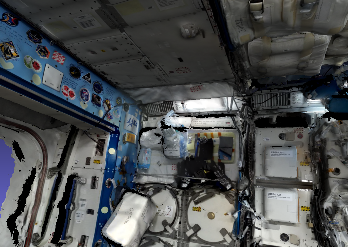
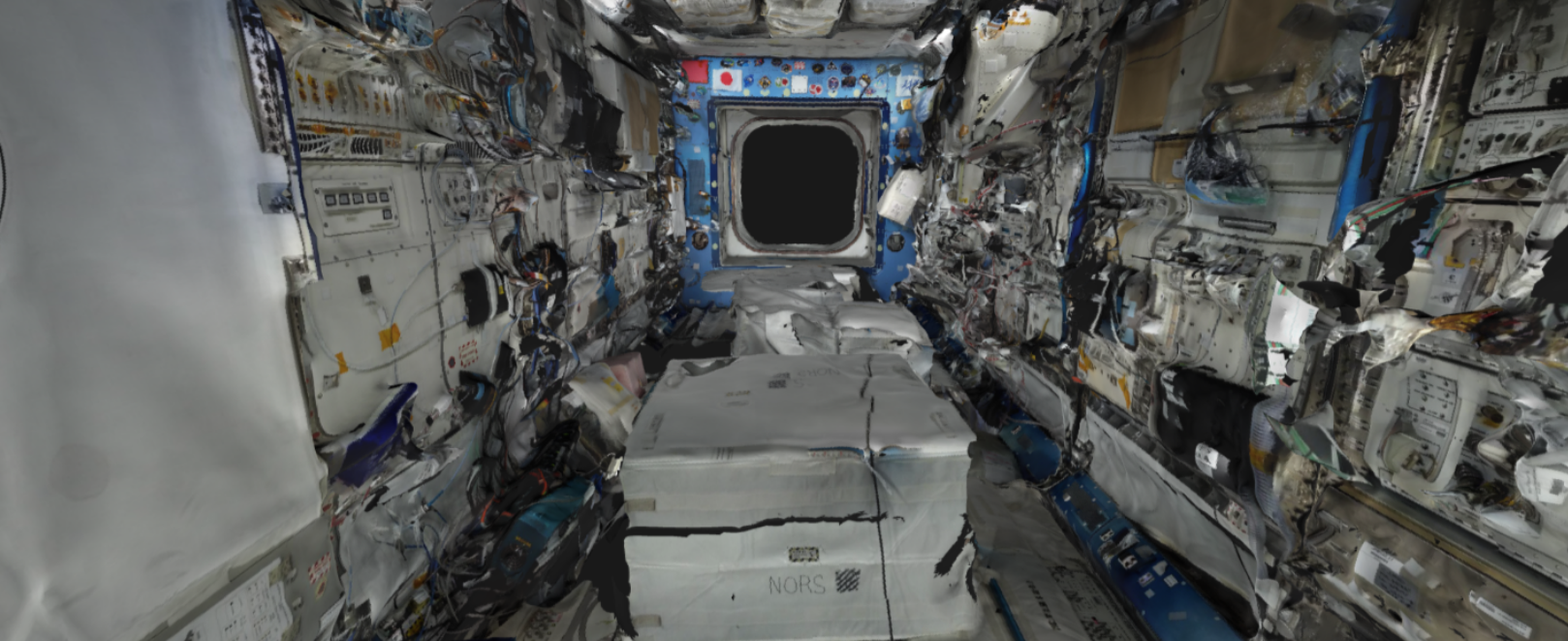
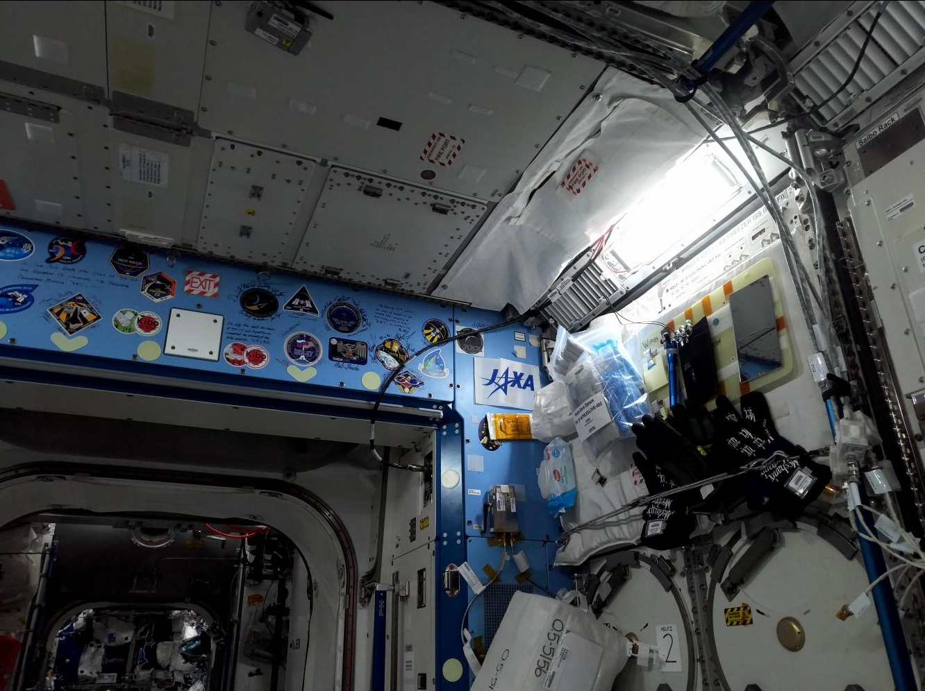
Fig. 10.1 A mesh created with the haz_cam depth + image sensor
and textured with sci_cam (top). A zoomed-out version showing
more of the module (middle). A sci_cam image that
was used to texture the mesh (bottom). The JEM module has many cables
and cargo, and the bot acquired the data spinning in place. This
resulted in some noise and holes in the mesh. The sci_cam texture was,
however, quite seamless, with very good agreement with the nav_cam
texture (not shown), which shows that the registration was done correctly.
10.2.2. Overview
Two Astrobee robots, named
bumble and queen, scanned the JEM, with each doing a portion. Both
robots have a wide-field of view navigation camera (nav_cam), a
color camera (sci_cam), and a low-resolution depth+intensity camera
(haz_cam).
To record the data, the robots took several stops along the center module axis, and at each stop acquired data from a multitude of perspectives, while rotating in place.
The data was combined into a sparse SfM map using theia_sfm
(Section 16.76). The camera poses were refined with
rig_calibrator (Section 16.60). That tool models the
fact that each set of sensors is on a rig (contained within a rigid
robot frame). Then, the depth clouds were fused into a mesh
with voxblox_mesh (Section 16.79), and textured with
texrecon (Section 16.75).
10.2.3. Data acquisition strategy
If designing a mapping approach, it is best to:
Have the cameras face the surface being imaged while moving parallel to it, in a panning motion.
Ensure consecutively acquired images have about 75% - 90% overlap. This and the earlier condition result in a solid perspective difference but enough similarity so that the images are registered successfully.
If more than one robot (rig) is used, there should be a decently-sized surface portion seen by more than rig, to be able to tie them reliably together.
10.2.4. Challenges
This example required care to address the in-place rotations, which
resulted in very little perspective change between nearby images
(hence in uncertain triangulated points), a wide range of resolutions
and distances, and occlusions (which resulted in holes). Another
difficulty was the low resolution and unique imaging modality of
haz_cam, which made it tricky to find interest point matches
(tie points) to other sensor data.
10.2.5. Data processing strategy
All sensors acquire the data at independent times. The color
sci_cam sensor takes one picture every few seconds, the
nav_cam takes about 2-3 pictures per second, and haz_cam takes
about 10 pictures per second.
The nav_cam sensor was chosen to be the reference sensor. A set
of images made by this sensor with both robots was selected, ideally
as in Section 10.2.3, and a Structure-from-Motion
sparse map was built.
Since the haz_cam sensor acquires images and depth data frequently
(0.1 seconds), for each nav_cam image the haz_cam frame
closest in time was selected and its acquisition timestamp was
declared to be the same as for the nav_cam. Even if this
approximation may result in the geometry moving somewhat, it is likely
to not be noticeable in the final textured mesh.
The same approximation is likely to be insufficient for sci_cam
when tying it to nav_cam, as the time gap is now larger, and it
can result in at least a few pixels of movement whose outcome
will be a very noticeable registration error.
The approach that rig_calibrator uses is to bracket each
sci_cam image by nav_cam images, as seen in
Section 10.1, followed by pose interpolation in
time. This however doubles the number of nav_cam images and the
amount of time for the various iterations that may be needed to refine
the processing. To avoid that, we use the following approach.
We assume that a reasonably accurate rig configuration file for the 2-rig 6-sensor setup already exists, but it may not be fully precise. It is shown in Section 10.2.13. It can be found as described in the previous paragraph, on a small subset of the data.
Then, given the SfM sparse map created with nav_cam only, the
haz_cam images (declared to be acquired at the same time as
nav_cam) were inserted into this map via the rig constraint. The
joint map was registered and optimized, while refining the rig
configuration (the transforms between rig sensors). A mesh was created
and textured, for each sensor. Any issues with mesh quality and
registration challenges can be dealt with at this time.
Then, the sci_cam images were also inserted via the rig
constraint, but not using nav_cam for bracketing, so the
placement was approximate. Lastly, the combined map was optimized,
while keeping the nav_cam and haz_cam poses fixed and refining
the sci_cam poses without the rig constraint or using the
timestamp information, which allows the sci_cam poses to move
freely to conform to the other already registered images.
This approach also helps with the fact that the sci_cam timestamp
can be somewhat unreliable, given that those images are acquired with
a different processor on the robot, so freeing these images from
the rig and time acquisition constraints helps with accuracy.
How all this is done will be shown in detail below.
10.2.6. Installing the software
See Section 2. The bin directory of the ASP software
should be added to the PATH environmental variable. Note that ASP
ships its own version of Python. That can cause conflicts if ROS
and ASP are run in the same terminal.
10.2.7. Data preparation
The Astrobee data is stored in ROS bags (with an exception for
sci_cam), with multiple bags for each robot.
10.2.7.1. sci_cam
The sci_cam data is not stored in bags, but as individual images,
for performance reasons, as the images are too big to publish over ROS.
Their size is 5344 x 4008 pixels. It is suggested to resample them
using the GDAL tool suite shipped with ASP (Section 16.25) as:
gdal_translate -r average -outsize 25% 25% -of jpeg \
  input.jpg output.jpg
The obtained images should be distributed in directories
corresponding to the robot, with names like my_data/bumble_sci
and my_data/queen_sci (Section 16.60.2).
10.2.7.3. haz_cam
As mentioned in Section 10.2.5, while the nav_cam
and sci_cam timestamps are kept precise, it makes the problem
much simpler to find the closest haz_cam images to the chosen
nav_cam images, and to change their timestamps to match nav_cam.
For that, the data should be extracted as follows:
ls my_data/bumble_nav/*.jpg > bumble_nav.txt
/usr/bin/python /path/to/ASP/libexec/extract_bag       \
--bag mybag.bag                                        \
--timestamp_list bumble_nav.txt                        \
--topics "/my/haz_intensity/topic /my/haz_depth/topic" \
--dirs "my_data/bumble_haz my_data/bumble_haz"         \
--timestamp_tol 0.2                                    \
--approx_timestamp
Notice several important differences with the earlier command. We use
the nav_cam timestamps for querying. The tolerance for how close
in time produced haz_cam timestamps are to input nav_cam
images is much smaller, and we use the option --approx_timestamp
to change the timestamp values (and hence the names of the produced
files) to conform to nav_cam timestamps.
This tool is called with two topics, to extract the intensity (image) and depth (point cloud) datasets, with the outputs going to the same directory (specified twice, for each topic). The format of the depth clouds is described in Section 16.60.14.
An analogous invocation should happen for the other rig, with the outputs going to subdirectories for those sensors.
10.2.8. A first small run
The strategy in Section 10.2.5 will be followed.
Consider a region that is seen in all nav_cam and haz_cam
images (4 sensors in total). We will take advantage of the fact that
each rig configuration is reasonably well-known, so we will create a
map with only the nav_cam data for both robots, and the other
sensors will be added later. If no initial rig configuration exists,
see Section 10.1.
10.2.8.1. The initial map
Create a text file having a few dozen nav_cam images from both
rigs in the desired region named small_nav_list.txt, with one
image per line. Inspect the images in eog. Ensure that each image
has a decent overlap (75%-90%) with some of the other ones, and they
cover a connected surface portion.
Run theia_sfm (Section 16.76) with the initial rig
configuration (Section 10.2.13), which we will
keep in a file called initial_rig.txt:
theia_sfm --rig-config initial_rig.txt \
  --image-list small_nav_list.txt      \
  --out-dir small_theia_nav_rig
The images and interest points can be examined in stereo_gui
(Section 16.72.9.4) as:
stereo_gui small_theia_nav_rig/cameras.nvm
10.2.8.2. Control points
The obtained map should be registered to world coordinates. Looking ahead, the full map will need registering as well, so it is good to collect control points over the entire module, perhaps 6-12 of them (the more, the better), with at least four of them in the small desired area of interest that is being done now. The process is described in Section 16.60.11. More specific instructions can be found in the Astrobee documentation.
If precise registration is not required, one could simply pick some visible object in the scene, roughly estimate its dimensions, and create control points based on that. The produced 3D model will then still be geometrically self-consistent, but the orientation and scale may be off.
We will call the produced registration files jem_map.pto and
jem_map.txt. The control points for the images in the future map
that are currently not used will be ignored for the time being.
10.2.8.3. Adding haz_cam
Create a list called small_haz_list.txt having the haz_cam images
with the same timestamps as the nav_cam images:
ls my_data/*_haz/*.jpg > small_haz_list.txt
Insert these in the small map, and optimize all poses together as:
float="bumble_nav bumble_haz queen_nav queen_haz"
rig_calibrator                                  \
  --registration                                \
  --hugin-file jem_map.pto                      \
  --xyz-file jem_map.txt                        \
  --use-initial-rig-transforms                  \
  --extra-list small_haz_list.txt               \
  --rig-config initial_rig.txt                  \
  --nvm small_theia_nav_rig/cameras.nvm         \
  --out-dir small_rig                           \
  --camera-poses-to-float "$float"              \
  --depth-to-image-transforms-to-float "$float" \
  --float-scale                                 \
  --intrinsics-to-float ""                      \
  --num-iterations 100                          \
  --export-to-voxblox                           \
  --num-overlaps 5                              \
  --min-triangulation-angle 0.5
The depth files will the same names but with the .pc extension will will be picked up automatically.
The value of --min-triangulation-angle filters out rays with a
very small angle of convergence. That usually makes the geometry more
stable, but if the surface is far from the sensor, and there is not
enough perspective difference between images, it may eliminate too many
features. The --max-reprojection-error option may eliminate
features as well.
Consider adding the option --bracket-len 1.0 that decides the length of
time, in seconds, between reference images used to bracket the other sensor. The
option --bracket-single-image will allow only one image of any non-reference
sensor to be bracketed.
It is suggested to carefully examine the text printed on screen by this tool. See Section 16.60.11 and Section 16.60.12 for the explanation of some statistics being produced and their expected values.
Then, compare the optimized configuration file
small_rig/rig_config.txt with the initial guess rig
configuration. The scales of the matrices in the
depth_to_image_transform fields for both sensors should remain
quite similar to each other, while different perhaps from their
initial values in the earlier file, otherwise the results later will
be incorrect. If encountering difficulties here, consider not
floating the scales at all, so omitting the --float-scale option
above. The scales will still be adjusted, but not as part of the
optimization but when the registration with control points
happens. Then they will be multiplied by the same factor.
Open the produced small_rig/cameras.nvm file in stereo_gui and
examine the features between the nav_cam and haz_cam
images. Usually they are very few, but hopefully at least some are
present.
Notice that in this run we do not optimize the intrinsics, only the camera poses and depth-to-image transforms. If desired to do so, optimizing the focal length may provide the most payoff, followed by the optical center. It can be tricky to optimize the distortion model, as one needs to ensure there are many features at the periphery of images where the distortion is strongest.
It is better to avoid optimizing the intrinsics unless the final texture has subtle misregistration, which may due to intrinsics. Gross misregistration is usually due to other factors, such as insufficient features being matched between the images. Or, perhaps, not all images that see the same view have been matched together.
Normally some unmodeled distortion in the images is tolerable if there are many overlapping images, as then their central areas are used the most, and the effect of distortion on the final textured mesh is likely minimal.
10.2.8.4. Mesh creation
The registered depth point clouds can be fused with voxblox_mesh
(Section 16.79):
cat small_rig/voxblox/*haz*/index.txt >       \
  small_rig/all_haz_index.txt

voxblox_mesh                                  \
  --index small_rig/all_haz_index.txt         \
  --output_mesh small_rig/fused_mesh.ply      \
  --min_ray_length 0.1                        \
  --max_ray_length 2.0                        \
  --median_filter '5 0.01'                    \
  --voxel_size 0.01
The first line combines the index files for the bumble_haz and
queen_haz sensors.
The produced mesh can be examined in meshlab. Normally it should
be quite seamless, otherwise the images failed to be tied properly
together. There can be noise where the surface being imaged has black
objects (which the depth sensor handles poorly), cables, etc.
Some rather big holes can be created in the occluded areas.
To not use all the input images and clouds, the index file passed in
can be edited and entries removed. The names in these files are in
one-to-one correspondence with the list of haz_cam images used
earlier.
The options --min_ray_length and --max_ray_length are used to
filter out depth points that are too close or too far from the sensor.
The mesh should be post-processed with the CGAL tools (Section 16.13). It is suggested to first remove most small connected components, then do some smoothing and hole-filling, in this order. Several iterations of may be needed, and some tuning of the parameters.
10.2.8.5. Texturing
Create the nav_cam texture with texrecon
(Section 16.75):
sensor="bumble_nav haz queen_nav"
texrecon                              \
--rig_config small_rig/rig_config.txt \
--camera_poses small_rig/cameras.txt  \
--mesh small_rig/fused_mesh.ply       \
--rig_sensor "${sensor}"              \
--undistorted_crop_win '1300 1200'    \
--skip_local_seam_leveling            \
--out_dir small_rig
The same can be done for haz_cam. Then reduce the undistorted crop
window to ‘250 200’. It is helpful to open these together in
meshlab and see if there are seams or differences between them.
To use just a subset of the images, see the --subset option. That
is especially important if the robot spins in place, as then some of
the depth clouds have points that are far away and may be less
accurate.
When working with meshlab, it is useful to save for the future
several of the “camera views”, that is, the perspectives from which
the meshes were visualized, and load them next time around. That is
done from the “Window” menu, in reasonably recent meshlab
versions.
10.2.8.6. Adding sci_cam
If the above steps are successful, the sci_cam images for the
same region can be added in, while keeping the cameras for the sensors
already solved for fixed. This goes as follows:
ls my_data/*_sci/*.jpg > small_sci_list.txt

float="bumble_sci queen_sci"
rig_calibrator                                  \
  --use-initial-rig-transforms                  \
  --nearest-neighbor-interp                     \
  --no-rig                                      \
  --bracket-len 1.0                             \
  --extra-list small_sci_list.txt               \
  --rig-config small_rig/rig_config.txt         \
  --nvm small_rig/cameras.nvm                   \
  --out-dir small_sci_rig                       \
  --camera-poses-to-float "$float"              \
  --depth-to-image-transforms-to-float "$float" \
  --intrinsics-to-float ""                      \
  --num-iterations 100                          \
  --export-to-voxblox                           \
  --num-overlaps 5                              \
  --min-triangulation-angle 0.5
The notable differences with the earlier invocation is that this time
only the sci_cam images are optimized (floated), the option
--nearest-neighbor-interp is used, which is needed since the
sci_cam images will not have the same timestamps as for the
earlier sensor, and the option --no-rig was added, which decouples
the sci_cam images from the rig, while still optimizing them with
the rest of the data, which is fixed and used as a constraint. The
option --bracket-len helps with checking how far in time newly
added images are from existing ones.
The texturing command is:
sensor="bumble_sci queen_sci"
texrecon                                    \
  --rig_config small_sci_rig/rig_config.txt \
  --camera_poses small_sci_rig/cameras.txt  \
  --mesh small_rig/fused_mesh.ply           \
  --rig_sensor "${sensor}"                  \
  --undistorted_crop_win '1300 1200'        \
  --skip_local_seam_leveling                \
  --out_dir small_sci_rig
Notice how we used the rig configuration and poses from
small_sci_rig but with the earlier mesh from small_rig. The
sensor names now refer to sci_cam as well.
The produced textured mesh can be overlaid on top of the earlier ones
in meshlab.
10.2.9. Results
See Section 10.2.
10.2.10. Scaling up the problem
If all goes well, one can map the whole module. Create several lists
of nav_cam images corresponding to different module portions. For
example, for the JEM, which is long in one dimension, one can
subdivide it along that axis.
Ensure that the portions have generous overlap, so many images show up in more than one list, and that each obtained group of images forms a connected component. That is to say, the union of surface patches as seen from all images in a group should be a contiguous surface.
For example, each group can have about 150-200 images, with 50-75 images being shared with each neighboring group. More images being shared will result in a tighter coupling of the datasets and in less registration error.
Run theia_sfm on each group of nav_cam images. A run can take
about 2 hours. While in principle this tool can be run on all images at
once, that may take longer than running it on smaller sets with
overlaps, unless one has under 500 images or so.
The obtained .nvm files can be merged with sfm_merge
(Section 16.63) as:
sfm_merge --fast_merge --rig_config small_rig/rig_config.txt \
  theia*/cameras.nvm --output_map merged.nvm
Then, given the large merged map, one can continue as earlier in the
document, with registration, adding haz_cam and sci_cam
images, mesh creation, and texturing.
10.2.11. Fine-tuning
If the input images show many perspectives and correspond to many distances from the surface being imaged, all this variety is good for tying it all together, but can make texturing problematic.
It is suggested to create the fused and textured meshes (using
voxblox_mesh and texrecon) only with subsets of the depth
clouds and images that are closest to the surface being imaged and
face it head-on. Both of these tools can work with a subset of the
data. Manual inspection can be used to delete the low-quality inputs.
Consider experimenting with the --median_filter,
--max_ray_length, and --distance_weight options in
voxblox_mesh (Section 16.79).
Some experimentation can be done with the two ways of creating
textures given by the texrecon option --texture_alg
(Section 16.75). The default method, named “center”, uses the
most central area of each image, so, if there are any seams when the
the camera is panning, they will be when transitioning from a surface
portion using one image to a different one. The other approach, called
“area”, tries for every small surface portion to find the camera whose
direction is more aligned with the surface normal. This may give
better results when imaging a round object from many perspectives.
In either case, seams are a symptom of registration having failed. It is likely because not all images seeing the same surface have been tied together. Or, perhaps the intrinsics of the sensors were inaccurate.
10.2.12. Surgery with maps
If a produced textured mesh is mostly good, but some local portion has artifacts and may benefit from more images and/or depth clouds, either acquired in between existing ones or from a new dataset, this can be done without redoing all the work.
A small portion of the existing map can be extracted with the
sfm_submap program (Section 16.65), having just nav_cam
images. A new small map can be made with images from this map and
additional ones using theia_sfm. This map can be merged into the
existing small map with sfm_merge --fast_merge
(Section 16.63). If the first map passed to this tool is the
original small map, its coordinate system will be kept, and the new
Theia map will conform to it.
Depth clouds for the additional images can be extracted. The combined
small map can be refined with rig_calibrator, and depth clouds
corresponding to the new data can be inserted, as earlier. The option
--fixed-image-list can be used to keep some images (from the
original small map) fixed to not change the scale or position of the
optimized combined small map.
These operations should be quite fast if the chosen subset of data is small.
Then, a mesh can be created and textured just for this data. If happy with the results, this data can then be merged into the original large map, and the combined map can be optimized as before.
10.2.13. Sample rig configuration
This is a rig configuration file having two rigs, with the
reference sensor for each given by ref_sensor_name.
The reference documentation is in Section 16.60.4.
ref_sensor_name: bumble_nav

sensor_name: bumble_nav
focal_length: 608
optical_center: 632.53683999999998 549.08385999999996
distortion_coeffs: 0.99869300000000005
distortion_type: fov
image_size: 1280 960
distorted_crop_size: 1200 900
undistorted_image_size: 1200 1000
ref_to_sensor_transform: 1 0 0 0 1 0 0 0 1 0 0 0
depth_to_image_transform: 1 0 0 0 1 0 0 0 1 0 0 0
ref_to_sensor_timestamp_offset: 0

sensor_name: bumble_haz
focal_length: 206.19094999999999
optical_center: 112.48999000000001 81.216598000000005
distortion_coeffs: -0.25949800000000001 -0.084849339999999995 0.0032980310999999999 -0.00024045673000000001
distortion_type: radtan
image_size: 224 171
distorted_crop_size: 224 171
undistorted_image_size: 250 200
ref_to_sensor_transform: -0.99936179050661522 -0.011924032028375218 0.033672379416940734 0.013367103760211168 -0.99898730194891616 0.042961506978788616 0.033126005078727511 0.043384190726704089 0.99850912854240503 0.03447221364702744 -0.0015773141724172662 -0.051355063495492494
depth_to_image_transform: 0.97524944805399405 3.0340999964032877e-05 0.017520679036474685 -0.0005022892199844 0.97505286059445628 0.026270283519653003 -0.017513503933106297 -0.02627506746113482 0.97489556315227599 -0.012739449966153971 -0.0033893213295227856 -0.062385053248766351
ref_to_sensor_timestamp_offset: 0

sensor_name: bumble_sci
focal_length: 1023.6054
optical_center: 683.97547 511.2185
distortion_coeffs: -0.025598438 0.048258987 -0.00041380657 0.0056673533
distortion_type: radtan
image_size: 1336 1002
distorted_crop_size: 1300 1000
undistorted_image_size: 1300 1200
ref_to_sensor_transform: 0.99999136796886101 0.0041467228570910052 0.00026206356569790089 -0.0041456529387620027 0.99998356891519313 -0.0039592248413610866 -0.00027847706785526265 0.0039581042406176921 0.99999212789968661 -0.044775738667823875 0.022844481744319863 0.016947323592326858
depth_to_image_transform: 1 0 0 0 1 0 0 0 1 0 0 0
ref_to_sensor_timestamp_offset: 0.0

ref_sensor_name: queen_nav

sensor_name: queen_nav
focal_length: 604.39999999999998
optical_center: 588.79561999999999 509.73835000000003
distortion_coeffs: 1.0020100000000001
distortion_type: fov
image_size: 1280 960
distorted_crop_size: 1200 900
undistorted_image_size: 1200 1000
ref_to_sensor_transform: 1 0 0 0 1 0 0 0 1 0 0 0
depth_to_image_transform: 1 0 0 0 1 0 0 0 1 0 0 0
ref_to_sensor_timestamp_offset: 0

sensor_name: queen_haz
focal_length: 210.7242
optical_center: 124.59857 87.888262999999995
distortion_coeffs: -0.37295935000000002 -0.011153150000000001 0.0029100743 -0.013234186
distortion_type: radtan
image_size: 224 171
distorted_crop_size: 224 171
undistorted_image_size: 250 200
ref_to_sensor_transform: -0.99983878639670731 -0.0053134634698496939 -0.017151335887125228 0.0053588429200665524 -0.99998225876857605 -0.0026009518744718949 -0.017137211538534192 -0.0026924438805366263 0.9998495220415089 0.02589135325068561 0.0007771584936297031 -0.025089928702394019
depth_to_image_transform: 0.96637484988953426 -0.0010183057117133798 -0.039142369279180113 0.00078683373128646066 0.96715045575148029 -0.005734923775739747 0.039147706343916511 0.0056983779719958138 0.96635836939244701 -0.0079348421014152053 -0.0012389803763148686 -0.053366194196969058
ref_to_sensor_timestamp_offset: 0

sensor_name: queen_sci
focal_length: 1016.3726
optical_center: 689.17409 501.88817
distortion_coeffs: -0.019654579 0.024057067 -0.00060629998 0.0027509131
distortion_type: radtan
image_size: 1336 1002
distorted_crop_size: 1300 1000
undistorted_image_size: 1300 1200
ref_to_sensor_transform: 0.99999136796886101 0.0041467228570910052 0.00026206356569790089 -0.0041456529387620027 0.99998356891519313 -0.0039592248413610866 -0.00027847706785526265 0.0039581042406176921 0.99999212789968661 -0.044775738667823875 0.022844481744319863 0.016947323592326858
depth_to_image_transform: 1 0 0 0 1 0 0 0 1 0 0 0
ref_to_sensor_timestamp_offset: 0