16.71. stereo_gui
The stereo_gui program is a GUI frontend to stereo and
parallel_stereo (Section 16.51). It can be used
for running stereo on small clips.
In addition, it can inspect the input images and produced datasets.
16.71.1. Use as stereo front-end
This program can be invoked just as parallel_stereo:
stereo_gui [options] <images> [<cameras>] output_prefix [dem]
Here is an example when using RPC cameras:
stereo_gui -t rpc left.tif right.tif left.xml right.xml run/run
One can zoom with the mouse wheel, or by dragging the mouse from
upper-left to lower-right (zoom in), and vice-versa (zoom out). The
= and - keys zoom in and out (also in the View menu). Use
the arrow keys to pan (first click to bring the image in focus).
By pressing the Control key while dragging the mouse, clips can be
selected in the input images, and then the stereo programs can be run
on these clips from the Run menu. The desired regions are passed
to these programs via the --left-image-crop-win and
--right-image-crop-win options. The actual command being used will
be displayed on screen, and can be re-run on a more powerful
machine/cluster without GUI access.
If the images are map-projected (Section 6.1.7), the low-resolution DEM will show up as the third image. There is no need to select a clip in that DEM.
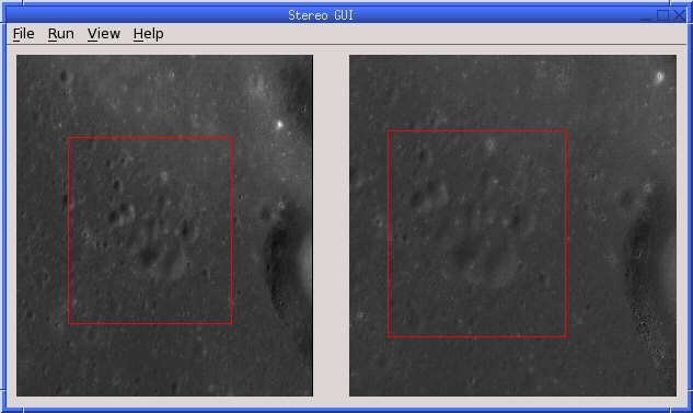
Fig. 16.34 An illustration of stereo_gui. Stereo processing will happen on
the regions selected by red rectangles.
If this program is invoked with two images (with or without cameras
and output prefix) and with values for --left-image-crop-win and
--right-image-crop-win, it will draw the corresponding regions on
startup.
See also our tutorials in Section 3.
16.71.2. Use as an image viewer
This program can be also used as a general-purpose image viewer, case in which no stereo options or cameras are necessary. It can display arbitrarily large images with integer, floating-point, or RGB pixels, including ISIS .cub files and DEMs. It handles large images by building on disk pyramids of increasingly coarser subsampled images and displaying the subsampled versions that are appropriate for the current level of zoom.
The images can be shown either all side-by-side (default), several
side-by-side (--view-several-side-by-side), as tiles on a grid
(using --grid-cols integer), or on top of each other (using
--single-window).
When the images are shown on top of each other, the option --use-georef will
overlay the images correctly if georeference information is present. In recent
builds this is the default, if all georeferences exist, and this mode can be
turned off with --no-georef.
It is possible to switch among the various display modes from the View menu.
When the images are shown side-by-side, the GUI can zoom in all images to the
same region, for easier comparison among them. This is accessible from the
View menu and with the option --zoom-all-to-same-region.
When the images are in a single window, an individual image can be turned on or off via a checkbox. Clicking on an image’s name will zoom to it and display it on top of other images. By right-clicking on an image name, other operations can be performed, such as hillshading, etc.
In this mode, the keys n and p can be used to cycle among
the images.
16.71.3. Other features
The stereo_gui program can:
Create and show hillshaded DEMs (Section 16.71.4).
Colorize images on-the-fly (
--colorize) and optionally show a colorbar with axes (--colorbar). See Section 16.71.5.Display the output of the ASP
colormapandhillshadetools (Section 16.14, Section 16.28).Overlay scatter plots on top of images (Section 16.71.6).
Overlay and edit polygons (Section 16.71.7).
Find pixel values and region bounds (Section 16.71.8).
View (Section 16.71.9) and edit (Section 16.71.11) interest point matches displayed on top of images.
Load .nvm files having an SfM solution (Section 16.71.9.4).
View ISIS
jigsawcontrol network files (Section 16.71.9.5).View GCP and .vwip files (Section 16.71.10).
Create GCP with georeferenced images and a DEM (Section 16.71.12).
Create interest point matches using mapprojected images (Section 16.71.13).
Threshold images (Section 16.71.14).
Cycle through images, showing one at a time (Section 16.71.15).
Save a screenshot to disk in the BMP or XPM format.
16.71.4. Hillshading
The stereo_gui program can create and display hillshaded DEMs. Example:
stereo_gui --hillshade dem.tif
Or, after the DEM is open, select from the GUI View menu the Hillshaded
images option.
Right-click to change the azimuth and elevation angles, hence the direction and height of the light source. Then toggle hillshading off and then on again.
Hillshaded images can also be produced with the hillshade tool
(Section 16.28) or with gdaldem hillshade (Section 16.25).
Images that are both colorized and hillshaded can be created with colormap
(Section 16.14), and then loaded in this program.
16.71.5. Displaying colorized images, with a colorbar and axes
stereo_gui can have images be colorized on-the-fly by mapping intensities to
colors of a given colormap. Optionally, a colorbar with axes (ticks) can be
shown next to each image.
CSV files can be colorized as well.
The --colorize and --colorbar flags are per-image with sticky semantics:
each applies to all subsequent images until turned off by --no-colorize or
--no-colorbar. The --colorbar flag implies --colorize.
An example invocation is as follows:
stereo_gui --colorbar              \
  --colormap-style inferno         \
  img1.tif                         \
  --colormap-style binary-red-blue \
  img2.tif                         \
  --no-colorbar                    \
  img3.tif
This will colorize the first two images (with colorbar) using the inferno
and binary-red-blue colormaps respectively. The third image is still
colorized (because --no-colorbar does not turn off colorization) but has
no colorbar. Use --no-colorize to fully turn off colorization. See
Section 16.14 for the full list of colormaps.
Each --colormap-style option also applies to all subsequent images until
overridden by this option with another value.
The range of intensities of each colorized image is computed automatically.
Right-click in each image to adjust this range. The --min and --max
options will set values for these that will apply to all images.
Colorization works as well with overlaid and georeferenced images.
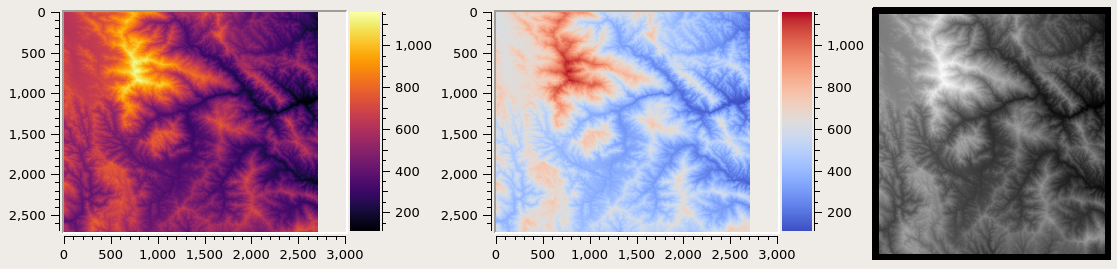
Fig. 16.35 An illustration of displaying images with specified colormap, with colorbar and axes, and without them. See Fig. 16.37 for an example having scattered points.
16.71.6. View scattered points
stereo_gui can plot and colorize scattered points stored in CSV files, and
overlay them on top of images or each other. Each point will show up as a dot
with a radius given by --plot-point-radius. Use --colorize or
--colorbar to enable colorization. A colorbar and axes can be shown as
well (Fig. 16.37).
Here is an example of plotting the final *pointmap.csv
residuals created by bundle_adjust for each interest point
(Section 16.5.11):
stereo_gui --colorize --colormap-style binary-red-blue \
  --min 0 --max 0.5 --plot-point-radius 2              \
  ba/run-final_residuals_pointmap.csv
This will use the longitude and latitude as the position, and will determine a color based on the 4th field in this file (the error) and the min and max values specified above (which correspond to blue and red in the colorized plot, respectively).
Files whose name contain the strings match_offsets and anchor_points
(created by bundle_adjust and jitter_solve, Section 16.38), and
error files created by pc_align (Section 16.53.9) can be plotted
the same way. Same with diff.csv files created by geodiff
(Section 16.26), only in the latter case the third (rather than fourth)
column will have the intensity (error) value.
The option --colormap-style accepts the same values as
colormap (Section 16.14).
To plot an arbitrary CSV file with longitude, latitude and value, do:
stereo_gui --csv-format "1:lon 2:lat 3:height_above_datum" \
  --datum D_MOON --colorize                                \
  filename.csv
If the file has data in projected units (such as using Easting and
Northing values), specify the option --csv-srs having the
projection, and use for the CSV format a string such as:
"1:easting 2:northing 3:height_above_datum"
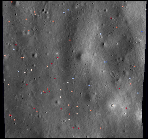
Fig. 16.36 A colorized CSV file overlaid on top of a georeferenced image.
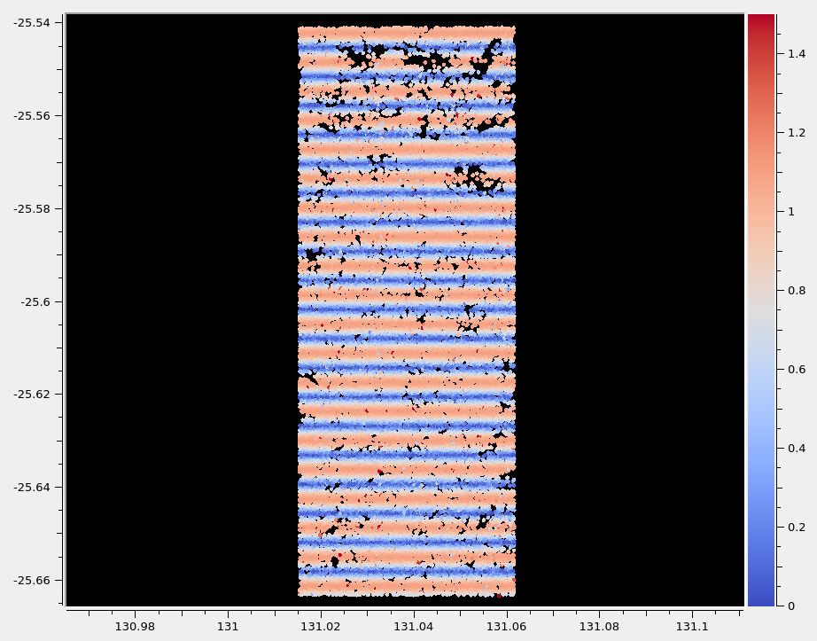
Fig. 16.37 A colorized CSV file with a colorbar and axes. This uses the --colorbar
option. Datasets with colorbars are displayed side-by-side
(Section 16.71.5).
16.71.7. Polygon editing and contouring
stereo_gui can be used to draw and edit polygonal shapes on top of
georeferenced images, save them as shape files (*.shp) or in plain text, and
load such files from the command line (including ones produced with external
tools). The editing functionality can be accessed by turning on polygon editing
from the Vector layer menu, and then right-clicking with the mouse to access
the various functions.
To create polygons, click with the left mouse button on points to be added. When clicking close to the starting point, the polygon becomes closed and and a new one can be drawn. A single point can be drawn by clicking twice in the same location. To draw a segment, click on its starting point, ending point, and then its starting point again. One must return to the starting point for the polygon to be recorded.
The resulting shapes can be saved from the right-click menu as shapefiles or in plain text. The shapefile specification prohibits having a mix of points, segments, and polygons in the same file, so all drawn shapes must be of the same kind.
When reading polygons and georeferenced images from disk, choose “View as georeferenced images” to plot the polygons on top of the images.
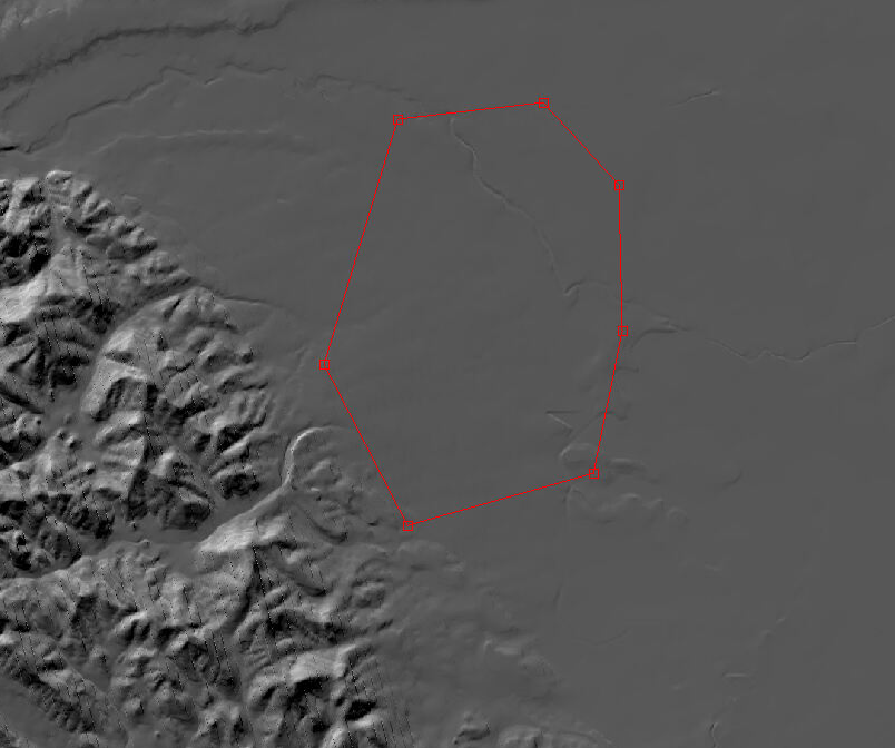
Fig. 16.38 A polygon drawn on top of a georeferenced image, in the “move vertices” editing mode.
16.71.7.1. Plain-text polygon files
The stereo_gui program can overlay plain-text polygon files on top of
images, such as:
stereo_gui --use-georef --single-window \
    poly1.txt poly2.txt image.tif
if each of these has georeference (and csv format) information. That is the case when the polygons were created in the GUI and saved to disk. This polygon format is described in Section 19.12.
To display polygons from any text file, additional options should be specified, such as:
stereo_gui --style poly --csv-format 1:lon,2:lat \
    --csv-datum D_MOON poly.csv
If such a file has multiple columns, the indices above can be changed to the ones desired to plot. Files having Easting-Northing information can be loaded as in Section 16.71.6, while omitting the third column in the csv format string.
If no georeference information exists, the CSV format can be
set to 1:x,2:y if it is desired to have the y axis point up, and
1:pix_x,2:pix_y if it should point down, so that such polygons
can be overlaid on top of images.
Any polygon properties set in the files will override the ones specified on the command line, to ensure that files with different properties can be loaded together.
16.71.7.2. Applications
The gdal_rasterize command can be used to keep or exclude the portion of a
given georeferenced image or a DEM that is within or outside a polygonal shape.
Example:
gdal_rasterize -i -burn <nodata_value> poly.shp dem.tif
Here, if the DEM nodata value is specified, the DEM will be edited and values outside the polygon will be replaced with no data.
The stereo_gui program can find the polygonal contour at a given image
threshold (which can be either set or computed from the Threshold menu).
This option is accessible from the Vector layer menu as well, with or
without the polygon editing mode on.
16.71.8. Finding pixel values and region bounds
When clicking on a pixel of an image opened in stereo_gui, the
pixel indices and image value at that pixel will be printed on screen.
When selecting a region by pressing the Control key while dragging
the mouse, the region pixel bounds (src win) will be displayed on
screen. If the image is geo-referenced, the extent of the region in
projected coordinates (proj win) and in the longitude-latitude
domain (lonlat win) will be shown as well.
The pixel bounds can be used to crop the image with gdal_translate
-srcwin (Section 16.25) and with the ISIS crop
command. The extent in projected coordinates can be used to crop
with gdal_translate -projwin, and is also accepted by
gdalwarp, point2dem, dem_mosaic, and mapproject,
for use with operations on regions.
One can zoom to a desired proj win from the View menu. This is helpful
to reproduce a zoom level. If multiple images are present,
the proj win used is for the first one. This can be invoked at startup
via --zoom-proj-win.
16.71.9. View interest point matches
stereo_gui can be used to view interest point matches (*.match
files), such as generated by ipmatch (Section 16.37),
bundle_adjust (Section 16.5), or
parallel_stereo. Several modes are supported.
16.71.9.1. View matches for an image pair
The match file to load can be specified via --match-file, or loaded
based on extension, so both of these will work:
stereo_gui left.tif right.tif            \
  --match-file run/run-left__right.match

stereo_gui left.tif right.tif run/run-left__right.match
The match file may also be auto-detected if stereo_gui was invoked like
parallel_stereo, with an output prefix:
stereo_gui left.tif right.tif run/run
and then the match file is loaded from the IP matches -> View IP matches
menu. (Auto-detection works only when the images are not
mapprojected, stereo was not run on image clips, and alignment method
is not epipolar or none.)
Plain-text match files (Section 19.10) can be loaded as:
stereo_gui           \
  --matches-as-txt   \
  left.tif right.tif \
  --match-file run/run-left__right.txt
These two options must be explicitly set, as otherwise the program may mistake the text file for a CSV file.
See also editing of interest point matches in Section 16.71.11.
16.71.9.2. View pairwise matches for N images
Given N images and interest point matches among any of them, such as
created by bundle_adjust, the options --pairwise-matches and
--pairwise-clean-matches (Section 16.71.17), also accessible
from the IP matches menu, can load the match file for a selected
image pair if the output prefix was specified. For that, run:
stereo_gui --pairwise-matches image1.tif ... imageN.tif run/run
then select a couple of images to view using the checkboxes on the left, and their match file will be displayed automatically.
This mode is available also from the View menu.
See an illustration in Fig. 16.39.
16.71.9.3. View all matches for N images
This mode allows viewing (and editing, see Section 16.71.11), interest points for N images at once, but some rigid and a bit awkward conventions are used, to be able to display all those points at the same time.
For image i, the match file must contain the matches from image i-1 to
i, or from image 0 to i. You can provide these match files to
stereo_gui by conforming to its naming convention
(output-prefix-fname1__fname2.match) or by selecting them from the
GUI when prompted. All match files must describe the same set of
interest points. The tool will check the positions of loaded points
and discard any that do not correspond to the already loaded points.
Run:
stereo_gui image1.tif ... imageN.tif run/run
(the last string is the output prefix). Select viewing of interest point matches.
If one of the match files fails to load or does not contain enough match points, the missing points will be added to an arbitrary position and flagged as invalid. You must either validate these points by manually moving them to the correct position or else delete them.
16.71.9.4. View NVM files
This tool can also visualize pairwise interest point matches loaded
from a plain-text .nvm file created by a Structure-from-Motion tool, such as
theia_sfm (Section 16.75) and rig_calibrator
(Section 16.60).
This file normally has all features shifted relative to the camera optical
center. Then an associated _offsets.txt file must exist having the optical
center per image. The above-mentioned programs write such an offset file. This
file is auto-loaded along with the .nvm file.
An .nvm file having features that are not shifted can be loaded as
well. Such files are created by rig_calibrator with the
--save_nvm_no_shift option (Section 16.60).
In this case, call stereo_gui with the additional option
--nvm-no-shift.
Example:
stereo_gui --nvm-no-shift --nvm nvm_no_shift.nvm
(The --nvm option can also be omitted, and only the file itself
can be specified.)
In this mode, the lowest-resolution subimage size is larger than
usual, to avoid creating small files. See
--lowest-resolution-subimage-num-pixels.
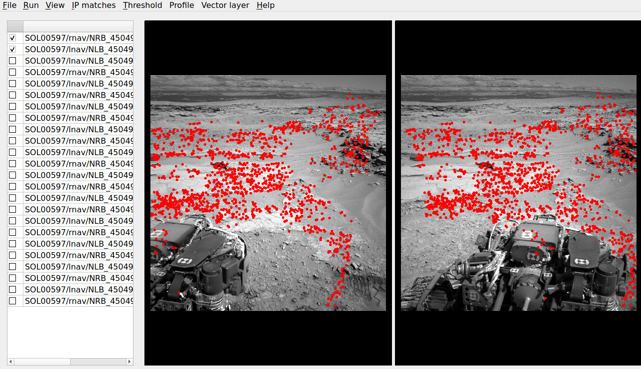
Fig. 16.39 An illustration of stereo_gui displaying an .nvm file.
Pairs of images can be chosen on the left, and matches will be shown.
The images were created with the MSL Curiosity rover (Section 10.3).
16.71.9.5. View ISIS control network files
The ISIS jigsaw (Section 12.3) binary control network format can be visualized as:
stereo_gui <image files> --isis-cnet <cnet file>
This file is expected to end with .net. The images must be the same as in the
control network, and in the same order, or else the results will be incorrect.
This file format does not keep track of the image names.
ASP’s bundle_adjust can also create and update such files
(Section 16.5.10). Then, non-ISIS images can be used as well, and this
tool can load the resulting control network.
16.71.10. View GCP and .vwip files
This tool can show the interest points from a GCP file (Section 16.5.9). Example:
stereo_gui image1.tif ... imageN.tif --gcp-file mygcp.gcp
This works even for a single image. If --gcp-file is not specified
but the GCP file is provided, this file will still be loaded.
Creating GCP is described in Section 16.71.12.
The stereo_gui program can also display .vwip files. Those are
interest points created by ipfind, bundle_adjust, or
parallel_stereo, before they are matched across images. One should
specify as many such files as images when launching this program.
16.71.11. Edit interest point matches
stereo_gui can be used to manually create and delete interest
point matches (useful in situations when automatic interest point
matching is unreliable due to large changes in illumination). This
works for N images.
Example:
stereo_gui image1.tif ... imageN.tif run/run
(the last string is the output prefix).
Select from the top menu:
IP matches -> View IP matches
If some matches exist already, they will be loaded, per
Section 16.71.9.3. Do not use
--pairwise-matches and --pairwise-clean-matches here.
Interest point matches can be created or deleted with the right-mouse click. This works whether a pre-existing match file was loaded, or starting from scratch.
To move interest points, right-click on an image and check “Move match point”. While this is checked, one can move interest points by clicking and dragging them within the image extent. Uncheck “Move match point” to stop moving interest points.
The edited interest point matches can be saved from the IP matches menu.
Section 16.5.10.1 describes the naming convention (both for
bundle_adjust and parallel_stereo). Then these programs will be able to
pick up the produced matches.
If handling N images at once becomes too complicated, it is suggested to edit the matches one pair at a time.
16.71.12. Creating GCP with with an orthoimage and a DEM
There exist situations when one has one or more images for which the camera files are either inaccurate or, for Pinhole camera models, just the intrinsics may be known.
Given a DEM of the area of interest, and optionally an orthoimage (mapprojected
image, georeferenced image), these an be used to create GCP files
(Section 16.5.9). GCP can be provided to bundle_adjust to refine the camera
poses, transform the cameras to given coordinates, or to create new
cameras (Section 16.5.9.2).
A DEM can be obtained using the instructions in Section 6.1.7.1.
Use, if applicable, dem_geoid to convert the DEM to be relative
to an ellipsoid.
Open the desired images, the orthoimage, the DEM, and the GCP file to be created in the GUI, as follows:
stereo_gui img1.tif img2.tif img3.tif \
  ortho.tif                           \
  --dem-file dem.tif                  \
  --gcp-file output.gcp               \
  --gcp-sigma 1.0                     \
  run/run
The orthoimage must be after the images for which GCP will be created. If no orthoimage exists, one can use the given DEM instead (and it can be hillshaded after loading to easier identify features).
The ground locations are found from the orthoimage and their elevations from the DEM. The interest points in the orthoimage are not saved to the GCP file.
A feature is identified and manually added as a matching interest point (match
point) in all open images, from left to right. For that, use the right
right-click menu, and select Add match point. This process is repeated a few
times. If the match point is not added in all images before starting with a new
one, that will result in an error. The match points can be moved around by
right-clicking to turn on this mode, and then dragging them with the mouse.
When done creating interest points, use the IP matches -> Write GCP file
menu item to save the GCP file. It is suggested to save the interest point
matches from the same menu, as later those can be edited and reused to create
GCP, while GCP cannot be edited.
If above the reference DEM and GCP file were not set, the GUI will prompt for their names.
If having many images, this process can be repeated for several small sets,
creating several GCP files that can then be passed together to bundle_adjust.
The sigmas for the GCP should be set via the option --gcp-sigma. Or use
bundle_adjust with the option --fix-gcp-xyz to ensure GCP are kept
fixed during optimization.
GCP can be visualized in stereo_gui (Section 16.71.10).
If the input images and the orthoimage are very similar visually, one can try to automatically detect and load interest point matches as follows:
ipfind img.tif ortho.tif
ipmatch img.tif ortho.tif
stereo_gui img.tif ortho.tif    \
  --match-file img__ortho.match \
  --dem-file dem.tif            \
  --gcp-file output.gcp         \
  --gcp-sigma 1.0
Then, the interest points can be inspected and edited as needed, and the GCP
file can be saved as above. See the documentation of ipfind
(Section 16.36) and ipmatch (Section 16.37), for how to increase the
number of matches, etc.
Lastly, non-GUI automatic approaches exists as well. Two methods are supported: tying a raw image to an orthoimage and a DEM (Section 16.24), and tying a produced DEM to a prior DEM (Section 16.18).
See earlier in this section for how GCP can be used.
16.71.13. Creating interest point matches using mapprojected images
To make it easier to create interest point matches in situations when the images are very different or taken from very diverse perspectives, the images can be first mapprojected onto a DEM, as then they look a lot more similar. The interest points are created among the mapprojected images, and the matches are transferred to the original images.
This section will describe how to do this with automatic and manual (GUI) means.
Given three images A.tif, B.tif, and C.tif,
cameras A.tsai, B.tsai, and C.tsai, and a DEM named dem.tif,
mapproject the images onto this DEM (Section 16.41), obtaining the images
A.map.tif, B.map.tif, and C.map.tif.
for f in A B C; do
    mapproject --tr 1.0 dem.tif $f.tif $f.tsai $f.map.tif
done
The same resolution (option --tr) should be used for all images, which should
be a compromise between the ground sample distance values for these images.
See Section 6.1.7 how how to find a DEM for mapprojection and other details.
Bundle adjustment will find interest point matches among the mapprojected images, and transfer them to the original images. Run:
bundle_adjust A.tif B.tif C.tif A.tsai B.tsai C.tsai          \
  --mapprojected-data 'A.map.tif B.map.tif C.map.tif dem.tif' \
  --min-matches 0 -o run/run
This will not recreate any existing match files either for mapprojected images or for unprojected ones. If that is desired, existing match files need to be deleted first.
Add options such as --ip-per-tile 250 --matches-per-tile 250 if needed to
increase the number of interest point matches.
If these images become too many to set on the command line, use the
options --image-list, --camera-list, --mapprojected-data-list
(Section 16.5.13).
The DEM at the end of this option is optional in the latest builds, if it can be looked up from the geoheader of the mapprojected images.
Each mapprojected image stores in its metadata the name of the original image, the camera model, the bundle-adjust prefix, if any, and the DEM it was mapprojected onto. Hence, the above command will succeed even if invoked with different cameras than the ones used for mapprojection, as long as the original cameras are still present and did not change.
If the mapprojected images are still too different for interest point matching among them to succeed, one can try to bring in more images that are intermediate in appearance or illumination between the existing ones, so bridging the gap.
Alternatively, interest point matching can be done manually in the GUI as follows:
stereo_gui --view-matches A.map.tif B.map.tif C.map.tif run/run
Interest points can be picked by right-clicking on the same feature in each
image, from left to right, and selecting Add match point. Repeat this
process for a different feature. The matches can be saved to disk from the menu.
The bundle adjustment command from above can be invoked to unproject the
matches. Do not forget to first delete first the match files among unprojected
images so that bundle_adjust can recreate them based on the projected
images.
Run:
stereo_gui --view-matches A.tif B.tif C.tif run/run
to check if the interest point matches, that were created using mapprojected
images, were correctly transferred to the original images. Consider using instead
the option --pairwise-matches if some features are not seen in all images.
See Fig. 16.40 for an illustration of this process.
It is suggested to use --mapprojected-data with --auto-overlap-params.
Then, the interest point matching will be restricted to the region of overlap
(expanded by the percentage in the latter option).
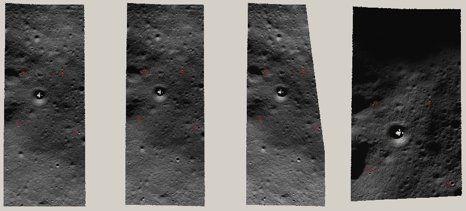
Fig. 16.40 An illustration of how interest points are picked manually for the purpose of bundle adjustment. This is normally not necessary if there exist images with intermediate illumination.
16.71.14. Image threshold
stereo_gui can be used to compute an image threshold for each of a
given set of images based on sampling pixels (useful for
shape-from-shading, see Section 11.1). This can be done by turning on
from the menu the Threshold detection mode, and then
clicking on pixels in the image. The largest of the chosen pixel
values will be set to the threshold for each image and printed
to the screen.
From the same menu it is possible to see or change the current threshold.
To highlight in the images the pixels at or below the image threshold,
select from the menu the View thresholded images option. Those
pixels will show up in red.
Related to this, if the viewer is invoked with --nodata-value
<double>, it will display pixels with values less than or equal to
this as transparent, and will set the image threshold to that no-data
value.
16.71.15. Cycle through images
To load only one image at a time, for speed, specify all images on the command
line, together with the --preview option. Then, can cycle through them with
the ‘n’ and ‘p’ keys.
In this mode, the lowest-resolution subimage size is larger than usual to avoid
creating small images when building an image pyramid. See
--lowest-resolution-subimage-num-pixels.
16.71.16. See also
The sfm_view tool (Section 16.66) can visualize cameras in orbit.
The asp_plot package (Section 6.3.1) can generate diagnostic plots and
PDF reports from ASP outputs.
The orbit_plot.py tool (Section 16.44) can visualize camera
orientations along an orbit.
16.71.17. Command line options for stereo_gui
Listed below are the options specific to stereo_gui. It will
accept all other parallel_stereo options as well.
- --grid-cols <integer (default: 1)>
Display images as tiles on a grid with this many columns.
- --window-size <integer integer (default: 1200 800)>
The width and height of the GUI window in pixels.
- -w, --single-window
Show all images in the same window (with a dialog to choose among them) rather than next to each other.
- --preview
Load and display the images one at a time, for speed. The ‘n’ and ‘p’ keys can be used to cycle through them.
- --view-several-side-by-side
View several images side-by-side, with a dialog to choose which images to show (also accessible from the View menu).
- --use-georef
Plot the images in the projected coordinate system given by the image georeferences. This is currently the default, and can be turned off with
--no-georefor from the View menu.- --nodata-value <double (default: NaN)>
Pixels with values less than or equal to this number are treated as no-data and displayed as transparent. This overrides the no-data values from input images.
- --hillshade
Interpret the input images as DEMs and hillshade them.
- --hillshade-azimuth
The azimuth value when showing hillshaded images.
- --hillshade-elevation
The elevation value when showing hillshaded images.
- --view-matches
Locate and display the interest point matches for a stereo pair. See also
--view-pairwise-matches,--view-pairwise-clean-matches.- --match-file
Display this match file instead of looking one up based on existing conventions (implies
--view-matches).- --pairwise-matches
Show images side-by-side. If just two of them are selected, load their corresponding match file, determined by the output prefix. Also accessible from the menu.
- --pairwise-clean-matches
Same as
--pairwise-matches, but use*-clean.matchfiles.- --nvm <string (default=””)>
Load this .nvm file having interest point matches. See also
--nvm-no-shift. Therig_calibratorprogram (Section 16.60) can create such files. This option implies--pairwise-matches.- --nvm-no-shift
Assume that the image features in the input nvm file were saved without being shifted to be relative to the optical center of the camera.
- --isis-cnet <string (default=””)>
Load a control network having interest point matches from this binary file in the ISIS jigsaw format. See also
--nvm.- --gcp-file
Display the GCP pixel coordinates for this GCP file (implies
--view-matches). Also save here GCP if created from the GUI. See also--gcp-sigma.- --gcp-sigma <double (default: 1.0)>
The sigma (uncertainty, in meters) to use for the GCPs (Section 16.5.9). A smaller sigma suggests a more accurate GCP. See also option
--fix-gcp-xyzinbundle_adjust(Section 16.5.13).- --dem-file
Use this DEM when creating GCP from images.
- --hide-all
Start with all images turned off (if all images are in the same window, useful with a large number of images).
- --zoom-proj-win <double double double double>
Zoom to this proj win on startup (Section 16.71.8). It is assumed that the images are georeferenced. Also accessible from the View menu. This implies
--zoom-all-to-same-region.- --zoom-all-to-same-region
Zoom all images to the same region. Also accessible from the View menu.
- --colorize
Colorize all images and/or CSV files after this option until
--no-colorizeis encountered. Per-image flag with sticky semantics (Section 16.71.5).- --no-colorize
Turn off colorization for subsequent images, until
--colorizeor--colorbaris encountered.- --colorbar
Colorize all images and/or CSV files after this option until
--no-colorbaris encountered, and show a colorbar with axes (Section 16.71.5). Implies--colorize. Right-click in each image to adjust the range of intensities to colorize.- --no-colorbar
Turn off the colorbar for subsequent images, until
--colorbaris encountered. Does not turn off colorization.- --colormap-style <string (default=”binary-red-blue”)>
Specify the colormap style. See Section 16.14 for options. Each style applies to all images after this option, until overridden by another instance of this option with a different value.
- --min <double (default = NaN)>
Value corresponding to ‘coldest’ color in the color map, when using
--colorizeor--colorbar, and plotting CSV data. Also used to manually set the minimum value in grayscale images. If not set, use the dataset minimum for color images, and estimate the minimum for grayscale images.- --max <double (default = NaN)>
Value corresponding to the ‘hottest’ color in the color map, when using
--colorizeor--colorbar, and plotting CSV data. Also used to manually set the maximum value in grayscale images. If not set, use the dataset maximum for color images, and estimate the maximum for grayscale images.- --plot-point-radius <integer (default = 2)>
When plotting points from CSV files, let each point be drawn as a filled ball with this radius, in pixels.
- --csv-format <string>
Specify the format of input CSV files as a list of entries column_index:column_type (indices start from 1). Examples:
1:x 2:y 3:z(a Cartesian coordinate system with origin at planet center is assumed, with the units being in meters),5:lon 6:lat 7:radius_m(longitude and latitude are in degrees, the radius is measured in meters from planet center),3:lat 2:lon 1:height_above_datum,1:easting 2:northing 3:height_above_datum(need to set--csv-srs; the height above datum is in meters). Can also use radius_km for column_type, when it is again measured from planet center. See Section 19.11 for details.- --csv-datum <string (default=””)>
The datum to use to to use when plotting a CSV file. Options: D_MOON (1,737,400 meters), D_MARS (3,396,190 meters), MOLA (3,396,000 meters), NAD83, WGS72, and NAD27. Also accepted: Earth (=WGS_1984), Mars (=D_MARS), Moon (=D_MOON).
- --csv-srs <string (default=””)>
The PROJ or WKT string to use when plotting a CSV file. If not specified, try to use the
--datumoption.- --lowest-resolution-subimage-num-pixels <integer (default: -1)>
When building a pyramid of lower-resolution versions of an image, the coarsest image will have no more than this many pixels. If not set, it will internally default to 1000 x 1000. This is increased to 10000 x 10000 when loading .nvm files or with the
--previewoption to avoid creating many small files.- --font-size <integer (default = 9)>
Set the font size.
- --no-georef
Do not use the georeference information when displaying the data, even when it exists. Also controllable from the View menu.
- --delete-temporary-files-on-exit
Delete any subsampled and other files created by the GUI when exiting.
- --create-image-pyramids-only
Without starting the GUI, build multi-resolution pyramids for the inputs, to be able to load them fast later. If used with
--hillshade, also build the hillshaded images and their multi-resolution pyramids.- --threads <integer (default: 0)>
Select the number of threads to use for each process. If 0, use the value in ~/.vwrc.
- --cache-size-mb <integer (default = 1024)>
Set the system cache size, in MB.
- --tile-size <integer (default: 256 256)>
Image tile size used for multi-threaded processing.
- --no-bigtiff
Tell GDAL to not create BigTiff files.
- --tif-compress <string (default = “LZW”)>
TIFF compression method. Options: None, LZW, Deflate, Packbits.
- -v, --version
Display the version of software.
- -h, --help
Display this help message.