9.1. About SfM
This chapter discusses how to create a terrain model (DEM) with Structure-from-Motion (SfM) if there exist two or more images and the camera models may not be fully known. This can be useful with aerial, hand-held, and historical images.
If the images have known metadata, such as stored in the EXIF header or from other sources, SfM can be avoided. That is discussed in the UAS example (Section 9.7).
If preexisting orthoimages and DEMs are available, it is possible to also avoid SfM by first creating a GCP file (Section 16.5.9) and then the camera models based on that (Section 9.5).
If the longitude and latitude of the corners of all images are known, see Section 16.8.
9.2. Camera solving overview
The camera_solve program (Section 16.12) offers several ways to
find the pose of frame camera images that do not come with any attached pose
metadata, or when information may be incomplete or inaccurate.
The camera_solve program is a Python script invoking two other
tools that we ship. The first of these is TheiaSfM. It generates initial camera position
estimates in a local coordinate space. The second one is bundle_adjust
(Section 16.5). This program improves the solution to account for
lens distortion and transforms the solution from local to global coordinates by
making use of additional input data.
The camera_solve program only solves for the extrinsic camera parameters
(camera position and orientation) and the user must provide intrinsic camera
information, such as focal length, optical center, and distortion parameters.
The camera_calibrate tool (see Section 16.10) can solve for
intrinsic parameters if you have access to the camera in question.
The rig_calibrator (Section 16.60) program can calibrate a rig
with one more cameras based on data acquired in situ, without a calibration
target. It can handle a mix of optical images and depth clouds. That program
has its own SfM script called theia_sfm (Section 16.75).
The bundle_adjust program can also solve for the intrinsics, without using a
rig or a calibration target. It can optionally constrain the solution against
a well-aligned prior terrain (Section 12.2.1).
The camera calibration information must be contained in a .tsai pinhole camera
model file and must passed in using the --calib-file option.
Section 9.5 has an example of a pinhole camera model file and discusses some heuristics for how to guess the intrinsics. A description of our supported pinhole camera models in Section 20.1.
In order to transform the camera models from local to world coordinates, one of three pieces of information may be used. These sources are listed below and described in more detail in the examples that follow:
A set of ground control points (Section 16.5.9). GCP can also be used to bypass SfM altogether, if there are many (Section 9.5).
A set of estimated camera positions (perhaps from a GPS unit) stored in a csv file (see Section 9.4).
A DEM or lidar datset that a local point cloud can be registered to using
pc_align(Section 16.53). This method can be more accurate if estimated camera positions are also used.
Power users can tweak the individual steps that camera_solve goes
through to optimize their results. This primarily involves setting up a
custom flag file for Theia and/or passing in settings to
bundle_adjust.
9.3. Example: Apollo 15 Metric Camera
9.3.1. Preparing the inputs
To demonstrate the ability of the Ames Stereo Pipeline to process a generic frame camera we use images from the Apollo 15 Metric camera. The calibration information for this camera is available online and we have accurate digital terrain models we can use to verify our results.
First, download with wget the two images at:
http://apollo.sese.asu.edu/data/metric/AS15/png/AS15-M-0114_MED.png
http://apollo.sese.asu.edu/data/metric/AS15/png/AS15-M-0115_MED.png
Convert these to TIF:
gdal_translate AS15-M-0114_MED.png AS15-M-0114_MED.tif
gdal_translate AS15-M-0115_MED.png AS15-M-0115_MED.tif
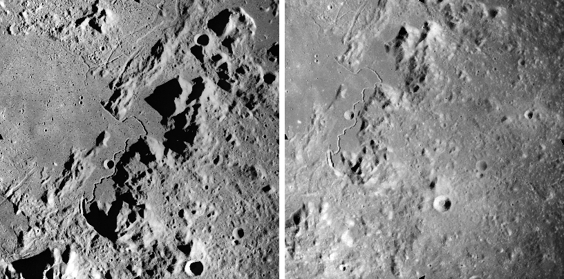
Fig. 9.1 The two Apollo 15 images
In order to make the example run faster we use downsampled versions of the original images. The images at those links have already been downsampled by a factor of \(4 \sqrt{2}\) from the original images. This means that the effective pixel size has increased from five microns (0.005 millimeters) to 0.028284 millimeters.
The next step is to fill out the rest of the pinhole camera model information we need, based on the Apollo 15 photographic equipment and mission summary report.
Looking at the ASP lens distortion models in Section 20.1, we see that the description matches ASP’s Brown-Conrady model. This model is, not recommended in general, as the distortion operation is slow (see a discussion in Section 20.1.2.4), but here we have to conform to what is expected.
Using the example in the appendix we can fill out the rest of the sensor model file (metric_model.tsai) so it looks as follows:
VERSION_4
PINHOLE
fu = 76.080
fv = 76.080
cu = 57.246816
cv = 57.246816
u_direction = 1  0  0
v_direction = 0  1  0
w_direction = 0  0  1
C = 0 0 0
R = 1 0 0 0 1 0 0 0 1
pitch = 0.028284
BrownConrady
xp = -0.006
yp = -0.002
k1 = -0.13361854e-5
k2 = 0.52261757e-09
k3 = -0.50728336e-13
p1 = -0.54958195e-06
p2 = -0.46089420e-10
phi = 2.9659070
These parameters use units of millimeters so we have to convert the nominal center point of the images from 2024 pixels to units of millimeters. Note that for some older images like these the nominal image center can be checked by looking for some sort of marking around the image borders that indicates where the center should lie. For these pictures there are black triangles at the center positions and they line up nicely with the center of the image. Before we try to solve for the camera positions we can run a simple tool to check the quality of our camera model file:
undistort_image AS15-M-0114_MED.tif metric_model.tsai \
  -o corrected_414.tif
It is difficult to tell if the distortion model is correct by using this
tool but it should be obvious if there are any gross errors in your
camera model file such as incorrect units or missing parameters. In this
case the tool will fail to run or will produce a significantly distorted
image. For certain distortion models the undistort_image tool may
take a long time to run.
If your input images are not all from the same camera or were scanned
such that the center point is not at the same pixel, you can run
camera_solve with one camera model file per input image. To do so
pass a space-separated list of files surrounded by quotes to the
--calib-file option such as
--calib-file "c1.tsai c2.tsai c3.tsai".
9.3.2. Creation of cameras in an arbitrary coordinate system
If we do not see any obvious problems we can go ahead and run the
camera_solve tool:
camera_solve out/ AS15-M-0114_MED.tif AS15-M-0115_MED.tif \
  --theia-overrides '--matching_strategy=CASCADE_HASHING' \
  --datum D_MOON --calib-file metric_model.tsai
The reconstruction can be visualized as:
view_reconstruction --reconstruction out/theia_reconstruction.dat
One may need to zoom out to see all cameras. See an illustration in Section 16.77.
Section 9.5 discusses how to avoid SfM altogether.
9.3.3. Creation of cameras in world coordinates
In order to generate a useful DEM, we need to move our cameras from local coordinates to global coordinates. The easiest way to do this is to obtain known ground control points (GCPs, Section 16.5.9) which can be identified in the frame images. This will allow an accurate positioning of the cameras provided that the GCPs and the camera model parameters are accurate.
We use stereo_gui to create GCP (Section 16.71.12). The input DEM is
generated from LRO NAC images. An arbitrary DEM for the desired planet can make
do for the purpose of transforming the cameras to plausible orbital coordinates.
(See Section 9.5 for more on GCP.)
For GCP to be usable, they can be one of two kinds. The preferred
option is to have at least three GCP, with each seen in at least two
images. Then their triangulated positions can be determined in local
coordinates and in global (world) coordinates, and bundle_adjust
will be able to compute the transform between these coordinate
systems, and convert the cameras to world coordinates.
The camera_solve program will automatically attempt this
transformation. This amounts to invoking bundle_adjust with the
option --transform-cameras-with-shared-gcp.
If this is not possible, then at least two of the images should have
at least three GCP each, and they need not be shared among the
images. For example, for each image the longitude, latitude, and
height of each of its four corners can be known. Then, one can pass
such a GCP file to camera_solve together with the flag:
--bundle-adjust-params "--transform-cameras-using-gcp"
This may not be as robust as the earlier approach. Consider the option
--fix-gcp-xyz, to not move the GCP during optimization.
Solving for cameras when using GCP:
camera_solve out_gcp/                                     \
  AS15-M-0114_MED.tif AS15-M-0115_MED.tif                 \
  --datum D_MOON --calib-file metric_model.tsai           \
  --theia-overrides '--matching_strategy=CASCADE_HASHING' \
  --gcp-file ground_control_points.gcp
Examine the lines ending in # GCP in the file:
out_gcp/asp_ba_out-final_residuals_pointmap.csv
(Section 16.5.11.5). If the residuals are no more than a handful pixels, and ideally less than a pixel, the GCP were used successfully.
Increase the value of --robust-threshold in bundle_adjust
(via --bundle-adjust-params in camera_solve)
if desired to bring down the big residuals in that file at the expense
of increasing the smaller ones. Consider also deleting GCP corresponding
to large residuals, as those may be inaccurate.
In recent ASP, one or more GCP files can be passed in without setting
--gcp-file. They should end in .gcp.
9.3.4. Running stereo
parallel_stereo                          \
  AS15-M-0114_MED.tif                    \
  AS15-M-0115_MED.tif                    \
  out_gcp/AS15-M-0114_MED.tif.final.tsai \
  out_gcp/AS15-M-0115_MED.tif.final.tsai \
  -t pinhole                             \
  --skip-rough-homography                \
  --stereo-algorithm asp_mgm             \
  --subpixel-mode 9                      \
  --sgm-collar-size 256                  \
  s_global/out
Create a terrain model and orthoimage:
point2dem -r moon                    \
  --stereographic --auto-proj-center \
  s_global/out-PC.tif                \
  --orthoimage s_global/out-L.tif    \
  --errorimage
See Section 16.51 and Section 16.56 for more information on the options used here.
The error image can be useful to see if the intrinsics are good. Big errors in the corners of the images may indicate that the intrinsics need refinement (Section 12.2.1).
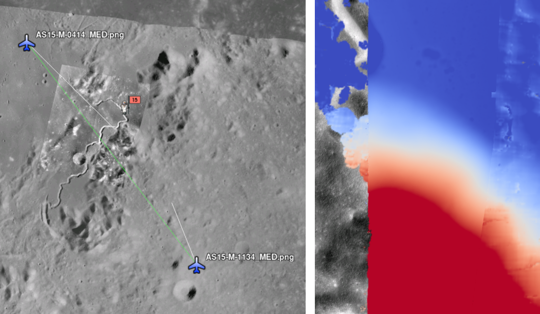
Fig. 9.2 Produced hillshaded DEM (left) and orthoimage (right). See Fig. 6.1 for a comparison of stereo algorithms.
Section 6 will discuss the parallel_stereo program
in more detail and the other tools in ASP.
9.3.5. Multiview reconstruction
The bundle_adjust program produces a report file having the convergence
angle and number of matches between any two images in a given set
(Section 16.5.11.4).
That data can be used to decide on promising stereo pairs to consider (Section 8.1). Pairwise stereo and DEM creation can be run, as in Section 3.
The DEMs can be mosaicked together with dem_mosaic (Section 16.20).
To give more weight in mosaicking to DEMs with a larger convergence angle,
see Section 16.20.2.4.
The input DEMs should agree quite well if the intrinsics are accurate, there is enough overlap between the images, many interest point matches were found, and the cameras were bundle-adjusted. Refining intrinsics is discussed in Section 12.2.1.
The produced mosaicked DEM (and cameras) can be aligned to a reference terrain with
pc_align (Section 16.53).
The creation of a fused mesh is discussed in Section 16.42.
9.4. Example: IceBridge DMS Camera
The DMS (Digital Mapping System) Camera is a frame camera flown on as part of the NASA IceBridge program, whose goal was to collect images of polar terrain.
The approach is, with a few exceptions, very similar to the one for the Apollo Metric camera.
The DMS images are available for download at the IceBridge ftp site. A list of the available data types can be found at the mission data summary page.
Several ways of creating cameras are discussed below, with or without SfM.
9.4.1. SfM approach
This example uses data from the November 5, 2009 flight over Antarctica. The following camera model (icebridge_model.tsai) was used (see Section 20.1 on Pinhole camera models):
VERSION_4
PINHOLE
fu = 28.429
fv = 28.429
cu = 17.9712
cv = 11.9808
u_direction = 1  0  0
v_direction = 0  1  0
w_direction = 0  0  1
C = 0 0 0
R = 1 0 0 0 1 0 0 0 1
pitch = 0.0064
Photometrix
xp = 0.004
yp = -0.191
k1 = 1.31024e-04
k2 = -2.05354e-07
k3 = -5.28558e-011
p1 = 7.2359e-006
p2 = 2.2656e-006
b1 = 0.0
b2 = 0.0
Note that these images are RGB format which is not supported by all ASP
tools. To use the files with ASP, first convert them to single channel
images using a tool such as ImageMagick’s convert,
gdal_translate, or gdal_edit.py. Different conversion methods
may produce slightly different results depending on the contents of your
input images. Some conversion command examples are shown below:
convert rgb.jpg -colorspace Gray gray.jpg
gdal_calc.py  --overwrite --type=Float32 --NoDataValue=-32768       \
  -A rgb.tif --A_band=1 -B rgb.tif --B_band=2 -C rgb.tif            \
  --C_band=3 --outfile=gray.tif --calc="A*0.2989+B*0.5870+C*0.1140"
gdal_translate -b 1 rgb.jpg gray.jpg
In the third command we used gdal_translate to pick a single band rather
than combining the three. This tool is shipped with ASP (Section 16.25).
Obtaining ground control points for icy locations on Earth can be particularly
difficult because they are not well surveyed or because the terrain shifts over
time. This may force you to use estimated camera positions to convert the local
camera models into global coordinates. To make this easier for IceBridge data
sets, ASP provides the icebridge_kmz_to_csv tool (see
Section 16.30) which extracts a list of estimated camera positions
(in ECEF coordinates) from the kmz files available for each IceBridge flight at
http://asapdata.arc.nasa.gov/dms/missions.html.
For such logic based on camera positions to work well, the camera positions must not be along a line, as then the 3D transform computed based on these positions will not be well-defined.
Another option which is useful when processing IceBridge data is the
--position-filter-dist option for bundle_adjust (measured in meters).
IceBridge data sets contain a large number of images and when processing many at
once you can significantly decrease your processing time by using this option to
limit interest-point matching to image pairs which are actually close enough to
overlap. A good way to determine what distance to use is to load the camera
position kmz file from their website into Google Earth and use the ruler tool to
measure the distance between a pair of frames that are as far apart as you want
to match.
Commands using these options may look like this:
icebridge_kmz_to_csv 1000123_DMS_Frame_Events.kmz \
  camera_positions.csv

camera_solve out                                          \
  2009_11_05_00667.JPG 2009_11_05_00668.JPG               \
  2009_11_05_00669.JPG 2009_11_05_00670.JPG               \
  2009_11_05_02947.JPG 2009_11_05_02948.JPG               \
  2009_11_05_02949.JPG 2009_11_05_02950.JPG               \
  2009_11_05_01381.JPG 2009_11_05_01382.JPG               \
  --theia-overrides '--matching_strategy=CASCADE_HASHING' \
  --datum WGS84 --calib-file icebridge_model.tsai         \
  --bundle-adjust-params                                  \
    '--no-datum
     --camera-positions camera_positions.csv
     --csv-format "1:file 2:lon 3:lat 4:height_above_datum"
     --position-filter-dist 0'
Run orbitviz (Section 16.45) to visualize the camera positions:
orbitviz out --load-camera-solve --hide-labels    \
 -r wgs84 -t nadirpinhole
9.4.2. Cameras from measurements
For some Earth missions the positions and orientations of the cameras are known. The cameras can then be found as in Section 16.8.1.7.
9.4.3. Cameras from GCP
See Section 9.5.
9.4.4. Cameras from orthoimages
Cameras can be created based on orthoimages, if available, such as for
IceBridge. The ortho2pinhole (Section 16.46) tool is used. Later,
the obtained cameras can be bundle-adjusted. Example for grayscale images:
ortho2pinhole raw_image.tif ortho_image.tif \
  icebridge_model.tsai output_pinhole.tsai
This needs the camera height above the datum. If not specified, it will be read from the orthoimage metadata, if set there. See this tool’s manual for more information.
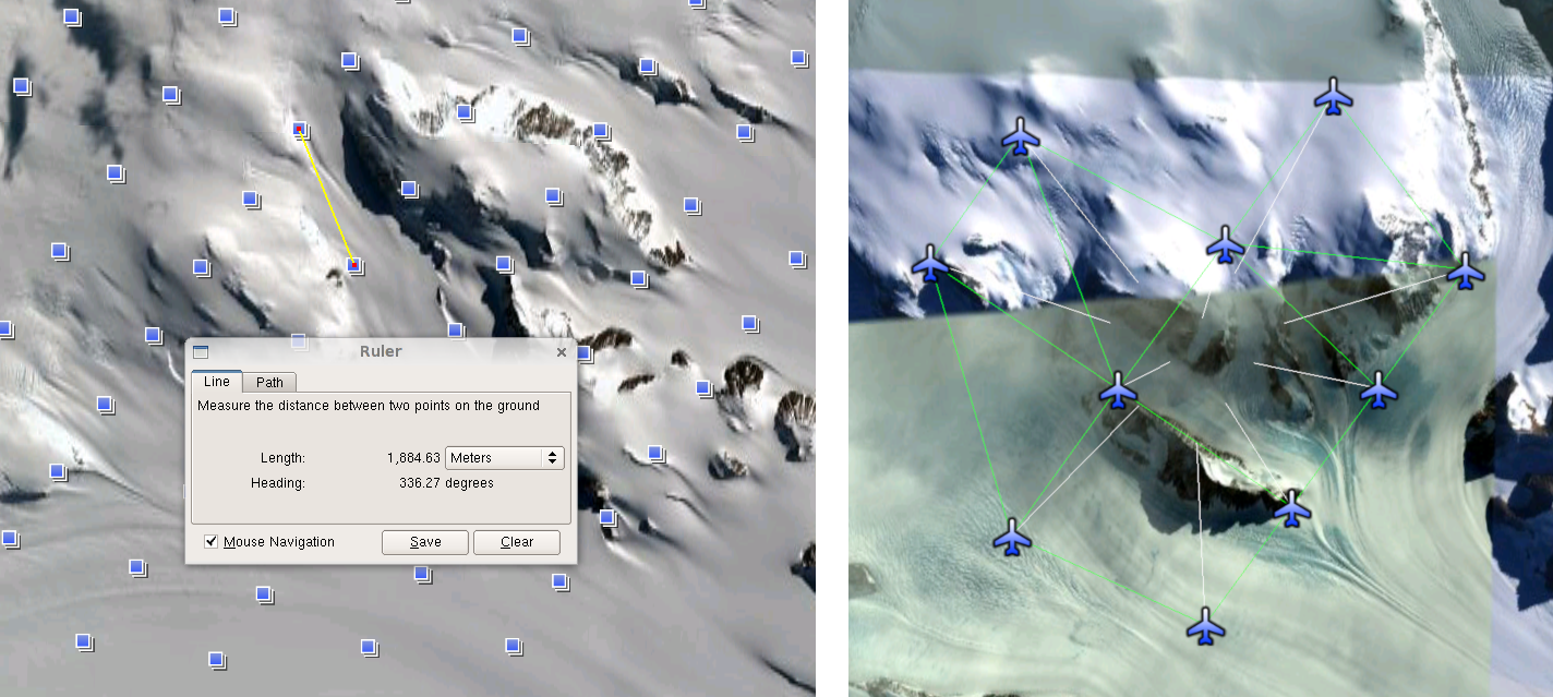
Fig. 9.3 Left: Measuring the distance between estimated frame locations using Google
Earth and an IceBridge kmz file. The kmz file is from the IceBridge website
with no modifications. A well-chosen position filter distance will mostly
limit image IP matching in this case to each image’s immediate “neighbors”.
Right: Display of camera_solve results for ten IceBridge images using
orbitviz.
Some IceBridge flights contain data from the Land, Vegetation, and Ice
Sensor (LVIS) lidar which can be used to register DEMs created using DMS
images. LVIS data can be downloaded at
ftp://n5eil01u.ecs.nsidc.org/SAN2/ICEBRIDGE/ILVIS2.001/. The lidar data
comes in plain text files that pc_align and point2dem can parse
using the following option:
--csv-format "5:lat 4:lon 6:height_above_datum"
ASP provides the lvis2kml tool to help visualize the coverage and
terrain contained in LVIS files, see Section 16.40
for details. The LVIS lidar coverage is sparse compared to the image
coverage and you will have difficulty getting a good registration unless
the region has terrain features such as hills or you are registering
very large point clouds that overlap with the lidar coverage across a
wide area. Otherwise pc_align will simply slide the flat terrain to
an incorrect location to produce a low-error fit with the narrow lidar
tracks. This test case was specifically chosen to provide strong terrain
features to make alignment more accurate but pc_align still failed
to produce a good fit until the lidar point cloud was converted into a
smoothed DEM.
9.4.5. Terrain creation
Run parallel_stereo (Section 16.51) on the DMS images:
parallel_stereo -t nadirpinhole       \
  --sgm-collar-size 256               \
  --skip-rough-homography             \
  --stereo-algorithm asp_mgm          \
  --subpixel-mode 9                   \
  --sgm-collar-size 256               \
  2009_11_05_02948.JPG                \
  2009_11_05_02949.JPG                \
  out/2009_11_05_02948.JPG.final.tsai \
  out/2009_11_05_02949.JPG.final.tsai \
  st_run/out
Create a DEM and orthoimage from the stereo results with point2dem
(Section 16.56):
point2dem --datum WGS_1984 \
  --auto-proj-center       \
  st_run/out-PC.tif        \
  --orthoimage st_run/out-L.tif
This will auto-guess an UTM or polar stereographic projection (Section 16.56.1).
Colorize and hillshade the DEM:
colormap --hillshade st_run/out-DEM.tif
Create a DEM from the LVIS data:
point2dem ILVIS2_AQ2009_1105_R1408_055812.TXT     \
  --datum WGS_1984                                \
  --auto-proj-center                              \
  --csv-format "5:lat 4:lon 6:height_above_datum" \
  --tr 30                                         \
  --search-radius-factor 2.0                      \
  -o lvis
How to combine multiple DEMs is described in Section 9.3.5.
9.4.6. Terrain alignment
Align the produced stereo point cloud to the LVIS data using pc_align
(Section 16.53):
pc_align --max-displacement 1000                         \
  st_run/out-DEM.tif ILVIS2_AQ2009_1105_R1408_055812.TXT \
  --csv-format "5:lat 4:lon 6:height_above_datum"        \
  --save-inv-transformed-reference-points                \
  --datum wgs84 --outlier-ratio 0.55                     \
  -o align_run/out
A DEM can be produced from the aligned point cloud, that can then be overlaid on top of the LVIS DEM.
For processing multiple images, see Section 9.3.5.
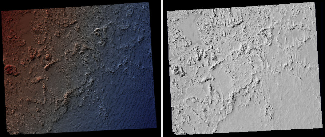
Fig. 9.4 A DEM and orthoimage produced with IceBridge data. The wavy artifacts in the bottom-right should go away if running a second-pass stereo with mapprojected images (Section 6.1.7), with a blurred version of this DEM as an initial guess.
Other IceBridge flights contain data from the Airborne Topographic
Mapper (ATM) lidar sensor. Data from this sensor comes packed in one of
several formats (variants of .qi or .h5) so ASP provides the
extract_icebridge_ATM_points tool to convert them into plain text
files, which later can be read into other ASP tools using the
formatting:
--csv-format "1:lat 2:lon 3:height_above_datum"
To run the tool, just pass in the name of the input file as an argument and a new file with a csv extension will be created in the same directory. Using the ATM sensor data is similar to using the LVIS sensor data.
For some IceBridge flights, lidar-aligned DEM files generated from the
DMS image files are available, see the web page here:
http://nsidc.org/data/iodms3 These files are improperly formatted and
cannot be used by ASP as is. To correct them, run the
correct_icebridge_l3_dem tool as follows:
correct_icebridge_l3_dem IODMS3_20120315_21152106_07371_DEM.tif \
  fixed_dem.tif 1
The third argument should be 1 if the DEM is in the northern hemisphere and 0 otherwise. The corrected DEM files can be used with ASP like any other DEM file.
Section 6 will discuss the parallel_stereo program
in more detail and the other tools in ASP.
9.5. Solving for pinhole cameras using GCP
A quick alternative to SfM with camera_solve is to create correctly oriented
cameras using ground control points (GCP, Section 16.5.9), an initial camera
having intrinsics only, and bundle adjustment. Here we outline this process.
9.5.1. GCP creation
Given the camera image, a similar-enough orthoimage, and a DEM, the gcp_gen
program (Section 16.24) can create a GCP file for it:
gcp_gen --camera-image img.tif \
  --ortho-image ortho.tif      \
  --dem dem.tif                \
  --output-prefix run/run      \
  --output-gcp gcp.gcp
If only a DEM is known, but in which one could visually discern roughly the same
features seen in the camera image, GCP can be created with point-and-click in
stereo_gui (Section 16.71.12). Such an input DEM can be found
as shown in Section 6.1.7.1. If the geolocations of image corners are
known, use instead cam_gen (Section 16.8).
9.5.2. Camera creation from GCP
We use the GCP to find the camera pose. For that, first create a Pinhole camera
(Section 20.1) file, say called init.tsai, with only the
intrinsics (focal length and optical center), and using trivial values for the
camera center and rotation matrix:
VERSION_4
PINHOLE
fu = 28.429
fv = 28.429
cu = 17.9712
cv = 11.9808
u_direction = 1  0  0
v_direction = 0  1  0
w_direction = 0  0  1
C = 0 0 0
R = 1 0 0 0 1 0 0 0 1
pitch = 0.0064
NULL
The entries fu, fv, cu, cv, amd pitch must be in the same
units (millimeters or pixels). When the units are pixels, the pixel pitch must
be set to 1.
The optical center can be half the image dimensions, and the focal length can be determined using the observation that the ratio of focal length to image width in pixels is the same as the ratio of camera elevation to ground footprint width in meters.
Here we assumed no distortion. Distortion can be refined later, if needed (Section 12.2.1).
For each camera image, run bundle adjustment with this data:
bundle_adjust -t nadirpinhole \
  img.tif init.tsai gcp.gcp   \
  --datum WGS84               \
  --inline-adjustments        \
  --init-camera-using-gcp     \
  --camera-weight 0           \
  --num-iterations 100        \
  --robust-threshold 2        \
  -o ba/run
This will write the desired correctly oriented camera file as
ba/run-init.tsai. The process can be repeated for each camera with an
individual output prefix.
The datum field must be adjusted depending on the planet.
9.5.3. Validation
It is very important to inspect the file:
ba/run-final_residuals_pointmap.csv
and look at the 4th column. Those will be the pixel residuals (reprojection error into cameras). They should be under a few pixels each, otherwise there is a mistake.
If bundle adjustment is invoked with a positive number of iterations, and with a small value for the robust threshold, it tends to optimize only some of the corners and ignore the others, resulting in a large reprojection error, which is not desirable. If however, this threshold is too large, it may try to optimize GCP that may be outliers, resulting in a poorly placed camera.
One can use the bundle adjustment option --fix-gcp-xyz to not
move the GCP during optimization, hence forcing the cameras to move more
to conform to them.
Validate the produced camera with mapproject:
mapproject dem.tif img.tif ba/run-init.tsai img.map.tif
and overlay the result on top of the DEM.
ASP provides a tool named cam_gen which can also create a pinhole
camera as above, and, in addition, is able to extract the heights of the
corners from a DEM (Section 16.8).
See also the bundle_adjust option --transform-cameras-with-shared-gcp.
This applies a wholesale transform to a self-consistent collection of cameras.
9.6. Refining the camera poses and intrinsics
The poses of the produced camera models can be jointly optimized with
bundle_adjust (Section 16.5).
Optionally, the intrinsics can be refined as well. Detailed recipes are in Section 12.2.1.
9.7. UAS example
The following example demonstrates how to produce camera models and a joint DEM from images taken by a UAS (Unmanned Aerial System). It is assumed that:
The images store in the EXIF metadata the camera center longitude, latitude, height above the datum, and yaw angle (the
GPSImgDirectionfield), relative to the North direction. Alternatively, this information (and perhaps also camera roll and pitch) is available in a list.The camera looks generally downward. This is not a strong assumption but makes it easier to determine which images overlap with which.
The camera is Frame (Pinhole) (Section 20.1), with known intrinsics. If those are not known, it is shown below how to estimate them and then refine them later.
The metadata is extracted from the EXIF header with the sfm_proc program
(Section 16.64):
ls images/*.JPG > images/image_list.txt
sfm_proc                             \
  --image-list images/image_list.txt \
  --out-dir cameras
This writes the file cameras/extrinsics.txt, having the above-mentioned
information. This file can also be created manually if the needed data are
stored in other ways.
The format of this file and how to use the cam_gen program to create the
camera models is shown in Section 16.8.1.7. That program needs the
camera intrinsics, including the focal length and optical center in pixel units,
and the lens distortion parameters.
If the focal length is not known, it is suggested to estimate it from the
FocalLengthIn35mmFilm field in the EXIF header, if available.
For example, if this has the value 46, and the image width is known
to be 9248 pixels, the following gives an estimate for the focal length in
pixels:
focal_length = 46.0 * 9248.0 / 35.0 = 12154.51428571
The optical center can be set to half the image dimensions. The lens distortion coefficients can be set to 0 for an initial estimate.
The produced rough camera models can be validated as shown in Section 16.8.3. That will require an external DEM, that can be found as described in Section 6.1.7.1, and which may need an adjustment as shown in Section 6.1.7.2.
The camera models can be refined with bundle_adjust with fixed intrinsics,
as shown in Section 12.2.2.3. The intrinsics can be refined later
(Section 12.2.1).
The images and produced cameras can be used to create and then merge DEMs, per Section 9.3.5.
The general Structure-from-Motion (SfM) approach is described in Section 9.1.