16.18. dem2gcp

This program generates GCP (Section 16.5.9) based on densely measuring the misregistration and/or warping between two DEMs, which helps correct these effects. The cause is usually inaccuracies in camera extrinsics or intrinsics, including lens distortion.

The approach is as follows. The dense disparity from an ASP-produced misregistered or warped DEM to a correct reference DEM is found. This program will take as input that disparity and interest point matches between the raw images, and will produce GCP with correct ground positions based on the reference DEM.

Bundle adjustment with intrinsics optimization (Section 12.2.1.2) or the jitter solver (Section 16.39) can then be invoked with the GCP to correct the issues.

This program was motivated by the processing of historical images (Section 8.26), particularly the KH-7 and KH-9 panoramic images.

16.18.1. ASP DEM creation

Prepare the images and camera models, such as in Section 8.28 or Section 8.27. This workflow expects the cameras to already incorporate any prior alignment or adjustments. Bundle adjustment (Section 16.5) can apply such transforms for Pinhole (Section 20.1), CSM (Section 8.12), and OpticalBar (Section 20.2) cameras.

Mapproject (Section 16.42) the images at the same appropriate resolution (close to native image GSD) onto the reference DEM.

Use a local projection for mapprojection, such as UTM or stereographic. Run stereo with the mapprojected images (Section 6.1.7). Use the asp_mgm algorithm with --subpixel-mode 9 (Section 6.1.1). This will ensure the best quality. If more than two images, pairwise stereo can be run and the DEMs can be mosaicked with dem_mosaic (Section 16.20).

Overlay the mapprojected images, produced DEM, and reference DEM in stereo_gui (Section 16.70). These should be roughly in the same place, but with some misregistration or warping.

Ensure parallel_stereo was invoked to generate dense matches from disparity (Section 12.2.4.2). It is suggested to use --num-matches-from-disparity 100000 or so. That is a very large number of interest points, but will help produce sufficient GCP later on.

The number of matches can be reduced later for bundle adjustment with the option --max-pairwise-matches, and fewer GCP can be created with dem2gcp as described below.

The dense match files should follow the naming convention for the original raw images (Section 16.5.10.1). Sufficiently numerous sparse matches, as produced by bundle adjustment, will likely work as well.

16.18.2. Comparison with the reference DEM

Fig. 16.3 A low-resolution KH-7 DEM produced by ASP (left) and a reference DEM (right). These must be visually similar and with enough features for dem2gcp to work. The DEMs can be overlaid to see if there is significant local warping.

Some hole-filling and blur can be applied to the ASP DEM with dem_mosaic (Section 16.20.2.6 and Section 16.20.2.9).

For example:

gdal_translate -r average -outsize 50% 50% dem.tif dem_small.tif

can reduce the resolution. This likely will do a better job than gdalwarp, which uses interpolation.

The two DEMs must be re-gridded to the same local projection and grid size. Example (adjust the projection center):

proj='+proj=stere +lat_0=27.909 +lon_0=102.226 +k=1 +x_0=0 +y_0=0 +datum=WGS84 +units=m +no_defs'
gdalwarp -tr 20 20 -t_srs "$proj" -r cubicspline dem_in.tif dem_out.tif

It is not required that the produced DEMs have precisely the same extent, but this is strongly advised. This helps with visualizing the disparity between the DEMs (see below) and allows for manual control of disparity via --corr-search (Section 14.4.2). The gdalwarp -te option can produce datasets with a given extent.

The DEMs should be hillshaded. It is suggested to use the GDAL (Section 16.25) hillshading method, as it is more accurate than ASP’s own hillshade (Section 16.28). Here’s an example invocation, to be applied to each DEM:

gdaldem hillshade   \
  -multidirectional \
  -compute_edges    \
  input_dem.tif     \
  output_dem_hill.tif

Inspect the hillshaded images in stereo_gui. They should be similar enough in appearance and with a good range of values.

Consider adjusting the lighting azimuth and elevation in the hillshade program to get good contrast. See the options -az and -alt in gdaldem hillshade, and -a and -e in ASP’s hillshade.

Find the dense disparity from the warped hillshaded DEM to the reference hillshaded DEM with ASP’s correlator mode (Section 16.17):

parallel_stereo              \
  --correlator-mode          \
  --stereo-algorithm asp_mgm \
  --subpixel-mode 9          \
  --ip-per-tile 500          \
  warped_hill.tif            \
  ref_hill.tif               \
  warp/run

The order of hillshaded images here is very important. Increase --ip-per-tile if not enough matches are found. One could consider experimenting with ASP’s various stereo algorithms (Section 6.1.1).

Inspect the bands of the produced disparity image warp/run-F.tif. This requires extracting the horizontal and vertical disparities, and masking the invalid values, as in Section 16.34.1.9. These can be visualized, for example, as follows:

stereo_gui --colorbar      \
  --min -100 --max 100     \
  warp/run-F_b1_nodata.tif \
  warp/run-F_b2_nodata.tif

16.18.3. Running dem2gcp

This command must be invoked with the warped ASP DEM and the reference DEM whose hillshaded versions were used to produce the disparity. Do not use here DEMs before cropping/regridding/blur applications, as those are not consistent with the disparity.

dem2gcp                                            \
  --warped-dem asp_dem.tif                         \
  --ref-dem ref_dem.tif                            \
  --warped-to-ref-disparity warp/run-F.tif         \
  --left-image left.tif                            \
  --right-image right.tif                          \
  --left-camera left.tsai                          \
  --right-camera right.tsai                        \
  --match-file dense_matches/run-left__right.match \
  --max-pairwise-matches 50000                     \
  --max-num-gcp 20000                              \
  --gcp-sigma 1.0                                  \
  --output-gcp out.gcp

Here we passed in the left and right raw images, the latest left and right camera models that produced the warped DEM, and the dense matches between the raw images.

If there are more than two images, the “warped” DEM can be produced, for example, by merging with dem_mosaic (Section 16.20) individual pairwise stereo DEMs (as long as these are consistent). Then, this program can be called for the full image set as in Section 16.18.5. Alternatively, this tool can be invoked pairwise for individual stereo DEMs, creating many GCP files.

The match file need not have dense matches. It is only assumed that there are many and well-distributed.

All produced GCP files should be passed together with all images and cameras to bundle_adjust, as shown below.

Consider using the option --max-disp if the disparity has portions that are not accurate, such as when the ASP DEM and reference DEM were acquired at different times and too much changed on the ground.

Note the options --max-num-gcp and --max-pairwise-matches above. These are off by default.

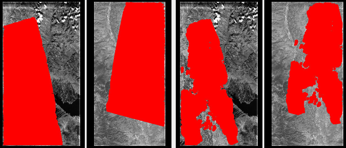
Fig. 16.4 Interest point matches (left, in red) and produced GCP (right), on top of the raw images. Flat areas do not have GCP. Plotted with stereo_gui (Section 16.70).

Plotted in Fig. 16.4 are the interest point matches and the resulting GCP. Their number is likely excessive here, though the bigger concern is if they are lacking over featureless terrain.

16.18.4. Solving for extrinsics and intrinsics

We employ the recipe from Section 12.2.1.3, that mostly addresses of the vertical component of disagreement between the ASP-produced and reference DEMs. The added GCP mostly address the horizontal component.

The most recent bundle-adjusted and aligned cameras can be converted to use the RPC lens distortion model (Section 20.1.2.8) as in Section 16.15. Or, the cameras can be used as is.

If solving for intrinsics and using RPC lens distortion, the small RPC coefficients must be changed manually to be at least 1e-7 in older builds, otherwise they will not get optimized. Here, RPC of degree 3 is used. A higher degree can be employed, either initially, or for subsequent iterations. In the latest builds this is done automatically by bundle_adjust (option --min-distortion).

The command when it is desired to refine the intrinsics as well:

bundle_adjust                                 \
  left_image.tif right_image.tif              \
  left_rpc_camera.tsai right_rpc_camera.tsai  \
  --inline-adjustments                        \
  --solve-intrinsics                          \
  --intrinsics-to-float all                   \
  --intrinsics-to-share none                  \
  --num-iterations 100                        \
  --match-files-prefix dense_matches/run      \
  --max-pairwise-matches 100000               \
  --remove-outliers-params '75.0 3.0 100 100' \
  --heights-from-dem ref_dem.tif              \
  --heights-from-dem-uncertainty 250          \
  out.gcp                                     \
  -o ba_rpc_gcp_ht/run

Note how we employ both the match file and the GCP created earlier. A higher value in --heights-from-dem-uncertainty gives less weight to the vertical constraint. Likely it is better to prioritize the GCP instead. Reducing --max-pairwise-matches will thin the interest point matches, but not the GCP.

This invocation can be sensitive to inaccurate GCP, as those do not use a robust cost function. Consider using the bundle_adjust option --max-gcp-reproj-err (Section 16.5.13) to remove worst GCP outliers. The option --max-disp for dem2gcp can help with this as well.

For linescan cameras, the jitter solver can be invoked instead with a very similar command to the above (Section 16.39).

Examine the pixel residuals before and after bundle adjustment (Section 16.5.11.5) in stereo_gui as:

stereo_gui --colorbar --min 0 --max 10             \
  ba_rpc_gcp_ht/run-initial_residuals_pointmap.csv \
  ba_rpc_gcp_ht/run-final_residuals_pointmap.csv

It should be rather obvious to see which residuals are from the GCP. These are also flagged in those csv files.

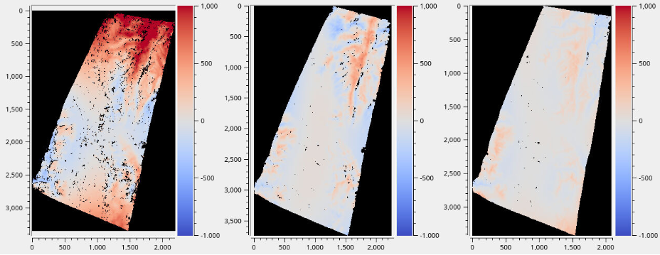
Fig. 16.5 Difference between the ASP DEM and reference DEM. The vertical range is -1000 m to 1000 m. From left-to-right: (a) no distortion modeling (b) modeling distortion with RPC of degree 3 and optimizing with --heights-from-dem (c) additionally, use the GCP produced by dem2gcp. The differences are found with geodiff (Section 16.26) and plotted with stereo_gui.

Fig. 16.6 The unwarped ASP DEM that results in the right-most difference in the above figure (within the green polygon), on top of the reference DEM.

Then, one can rerun stereo with the optimized cameras and the original images (again with the option --prev-run-prefix, or by doing a new run from scratch). The results are in Fig. 16.5. The warping is much reduced but not eliminated.

We further improved the results for KH-7 and KH-9 cameras by creating linescan cameras (Section 16.8.1.6) and running jitter_solve with GCP (Section 16.39).

16.18.5. Multiple images and cameras

This program can work with multiple images, cameras, and match files, as long as the “warped” DEM is consistent with these datasets. In particular, this DEM can even be produced with Shape-from-Shading (Section 16.67).

The match files can be specified via --match-files-prefix or --clean-match-files-prefix, in the manner of bundle_adjust (Section 16.5.10.1).

dem2gcp                                    \
  --warped-dem asp_dem.tif                 \
  --ref-dem ref_dem.tif                    \
  --warped-to-ref-disparity warp/run-F.tif \
  --image-list image_list.txt              \
  --camera-list camera_list.txt            \
  --clean-match-files-prefix matches/run   \
  --max-pairwise-matches 50000             \
  --max-num-gcp 100000                     \
  --gcp-sigma 1.0                          \
  --output-gcp out.gcp

Here, the entries in the camera list are usually after bundle adjustment, and the matches/run prefix points to the interest point matches, such as produced by bundle_adjust, or with dense matching (Section 12.2.4.2).

The value of --gcp-sigma should be a fraction of the ground sample distance (in meters), to ensure that GCP provide strong constraints in bundle adjustment.

The value in --max-pairwise-matches can be reduced if there is a large number of pairs of images.

The produced GCP file can then be passed to bundle_adjust or jitter_solve with the same lists of images, cameras, and match files.

16.18.6. Command-line options

--warped-dem <string (default: “”)>

The DEM file produced by stereo, that may have warping due to unmodeled distortion.

--ref-dem <string (default: “”)>

The reference DEM file, which is assumed to be accurate.

--warped-to-ref-disparity <string (default: “”)>

The stereo disparity from the warped DEM to the reference DEM (use the first band of the hillshaded DEMs as the inputs for the disparity).

--left-image <string (default: “”)>

The left raw image that produced the warped DEM.

--right-image <string (default: “”)>

The right raw image that produced the warped DEM.

--left-camera <string (default: “”)>

The left camera that was used for stereo.

--right-camera <string (default: “”)>

The right camera that was used for stereo.

--match-file <string (default: “”)>

The match file between the left and right raw images.

--image-list <string (default: “”)>

A file containing the list of images, when they are too many to specify on the command line. Use space or newline as separator. See also --camera-list.

--camera-list <string (default: “”)>

A file containing the list of cameras, when they are too many to specify on the command line. If the images have embedded camera information, such as for ISIS, this file may be omitted, or specify the image names instead of camera names.

--match-files-prefix <string (default: “”)>

Use the match files with this prefix.

--clean-match-files-prefix <string (default: “”)>

Use as input *-clean.match files with this prefix.

--max-pairwise-matches <int (default: -1)>

If positive, reduce the number of matches to load from any given match file to at most this value.

--gcp-sigma <double (default: 1.0)>

The sigma to use for the GCP points. A smaller value will give to GCP more weight. This should be a fraction of the image ground sample distance. Measured in meters. See also --gcp-sigma-image.

--output-gcp <string (default: “”)>

The produced GCP file with ground coordinates from the reference DEM.

--max-num-gcp <int (default: -1)>

The maximum number of GCP to write. If negative, all GCP are written. If more than this number, a random subset will be picked. The same subset will be selected if this program is called again.

--max-disp <double (default: -1.0)>

If positive, flag a disparity whose norm is larger than this as erroneous and do not use it for creating GCP. Measured in pixels. See also option --max-gcp-reproj-err in bundle_adjust (Section 16.5.13).

--gcp-sigma-image <string (default: “”)>

Given a georeferenced image with float values, for each GCP find its location in this image and closest pixel value. Let the GCP sigma be that value. Skip GCP that result in values that are no-data or are not positive. This overrides --gcp-sigma.

--search-len <int (default: 0)>

How many DEM pixels to search around to find a valid DEM disparity (pick the closest). This may help with a spotty disparity but should not be overused.

-v, --version

Display the version of software.

-h, --help

Display this help message.