8.26. Declassified satellite images: KH-4B

ASP has preliminary support for the declassified high-resolution CORONA KH-4B images.

This support is very experimental, and likely a lot of work is needed to make it work reliably.

For the latest suggested processing workflow, in the context of KH-9 images, see Section 8.28.

These images can be processed using either optical bar (panoramic) camera models or as pinhole camera models with RPC distortion. Most of the steps are similar to the example in Fig. 8.38. The optical bar camera model is based on [SCS03] and [SKY04], whose format is described in Section 20.2. For KH-9 images, the Improvements suggested in [GBRB22] are incorporated (Section 8.28.3).

8.26.1. Fetching the data

KH-4B images are available via the USGS Earth Explorer, at

https://earthexplorer.usgs.gov/

(an account is required to download the data). We will work with the KH-4B image pair:

DS1105-2248DF076
DS1105-2248DA082

To get these from Earth Explorer, click on the Data Sets tab and select the three types of declassified data available, then in the Additional Criteria tab choose Declass 1, and in the Entity ID field in that tab paste the above frames (if no results are returned, one can attempt switching above to Declass 2, etc). Clicking on the Results tab presents the user with information about these frames.

Clicking on Show Metadata and Browse for every image will pop-up a table with meta-information. That one can be pasted into a text file, named for example, DS1105-2248DF076.txt for the first image, from which later the longitude and latitude of each image corner will be parsed. Then one can click on Download Options to download the data.

8.26.2. Resizing the images

Sometimes the input images can be so large, that either the ASP tools or the auxiliary ImageMagick convert program will fail, or the machine will run out of memory.

It is suggested to resize the images to a more manageable size, at least for initial processing. This is easiest to do by opening the images in stereo_gui (Section 16.70), which will create a pyramid of subsampled (“sub”) images at 1/2 the full resolution, then 1/4th, etc. This resampling is done using local averaging, to avoid aliasing effects.

Alternatively, one can call gdal_translate (Section 16.25), such as:

gdal_translate -outsize 25% 25% -r average input.tif output.tif

This will reduce the image size by a factor of 4. The -r average option will, as before, help avoid aliasing.

A camera model (pinhole or optical bar) created at one resolution can be converted to another resolution by adjusting the pitch parameter (a higher value of pitch means bigger pixels so lower resolution). For optical bar cameras the image dimensions and image center need to be adjusted as well, as those are in units of pixels.

8.26.3. Stitching the images

Each downloaded image will be made up of 2-4 portions, presumably due to the limitations of the scanning equipment. They can be stitched together using ASP’s image_mosaic tool (Section 16.35).

For some reason, the KH-4B images are scanned in an unusual order. To mosaic them, the last image must be placed first, the next to last should be second, etc. In addition, as seen from the tables of metadata discussed earlier, some images correspond to the Aft camera type. Those should be rotated 180 degrees after mosaicking, hence below we use the --rotate flag for that one. The overlap width is manually determined by looking at two of the sub images in stereo_gui.

With this in mind, image mosaicking for these two images will happen as follows:

image_mosaic DS1105-2248DF076_d.tif DS1105-2248DF076_c.tif \
  DS1105-2248DF076_b.tif  DS1105-2248DF076_a.tif           \
  -o DS1105-2248DF076.tif                                  \
  --ot byte --overlap-width 7000 --blend-radius 2000
image_mosaic DS1105-2248DA082_d.tif DS1105-2248DA082_c.tif \
  DS1105-2248DA082_b.tif  DS1105-2248DA082_a.tif           \
  -o DS1105-2248DA082.tif                                  \
  --ot byte --overlap-width 7000 --blend-radius 2000       \
  --rotate

In order to process with the optical bar camera model these images need to be cropped to remove the most of empty area around the image. The four corners of the valid image area can be manually found by clicking on the corners in stereo_gui. Note that for some input images it can be unclear where the proper location for the corner is due to edge artifacts in the film. Do your best to select the image corners such that obvious artifacts are kept out and all reasonable image sections are kept in.

ASP provides a simple Python tool called historical_helper.py to rotate the image so that the top edge is horizontal while also cropping the boundaries. This tool requires installing the ImageMagick software. See Section 16.29 for more details.

Pass in the corner coordinates as shown below in the order top-left, top-right, bot-right, bot-left (column then row). This is also a good opportunity to simplify the file names going forwards.

historical_helper.py rotate-crop                                     \
  --interest-points '4523 1506  114956 1450  114956 9355  4453 9408' \
  --input-path DS1105-2248DA082.tif                                  \
  --output-path aft.tif
historical_helper.py rotate-crop                                     \
  --interest-points '6335 1093  115555 1315  115536 9205  6265 8992' \
  --input-path DS1105-2248DF076.tif                                  \
  --output-path for.tif

See Section 8.26.2 if these steps failed, as perhaps the images were too large.

8.26.4. Fetching a ground truth DEM

To create initial cameras to use with these images, and to later refine and validate the terrain model made from them, we will need a ground truth source. Several good sets of DEMs exist, including SRTM, ASTER, and TanDEM-X (Section 6.1.7.1). Here we will work with SRTM, which provides DEMs with a 30-meter grid size. The bounds of the region of interest are inferred from the tables with meta-information from above.

The SRTM DEM must be adjusted to be relative to the WGS84 datum, as discussed in Section 6.1.7.2.

The visualization of all images and DEMs can be done in stereo_gui.

8.26.5. Creating camera files

ASP provides the tool named cam_gen (Section 16.8) that, based on a camera’s intrinsics and the positions of the image corners on Earth’s surface will create initial camera models that will be the starting point for aligning the cameras.

To create optical bar camera models, an example camera model file is needed. This needs to contain all of the expected values for the camera, though image_size, image_center, iC, and IR can be any value since they will be recalculated. The pitch is determined by the resolution of the scanner used, which is seven microns. The other values are determined by looking at available information about the satellite. For the first image (DS1105-2248DF076) the following values were used:

VERSION_4
OPTICAL_BAR
image_size = 13656 1033
image_center = 6828 517
pitch = 7.0e-06
f = 0.61000001430511475
scan_time = 0.5
forward_tilt = 0.2618
iC = -1030862.1946224371 5468503.8842079658 3407902.5154047827
iR = -0.95700845635275322 -0.27527006183758934 0.091439638698163225 -0.26345593052063937 0.69302501329766897 -0.67104940475144637 0.1213498543172795 -0.66629027007731101 -0.73575232847574434
speed = 7700
mean_earth_radius = 6371000
mean_surface_elevation = 4000
motion_compensation_factor = 1.0
scan_dir = right

For a description of each value, see Section 20.2. For the other image (aft camera) the forward tilt was set to -0.2618 and scan_dir was set to ‘left’. The correct values for scan_dir (left or right) and use_motion_compensation (1.0 or -1.0) are not known for certain due to uncertainties about how the images were recorded and may even change between launches of the KH-4 satellite. You will need to experiment to see which combination of settings produces the best results for your particular data set.

The metadata table from Earth Explorer has the following entries for DS1105-2248DF076:

NW Corner Lat dec   31.266
NW Corner Long dec  99.55
NE Corner Lat dec   31.55
NE Corner Long dec  101.866
SE Corner Lat dec   31.416
SE Corner Long dec  101.916
SW Corner Lat dec   31.133
SW Corner Long dec  99.55

These correspond to the upper-left, upper-right, lower-right, and lower-left pixels in the image. We will invoke cam_gen as follows:

cam_gen --sample-file sample_kh4b_for_optical_bar.tsai     \
  --camera-type opticalbar                                 \
  --lon-lat-values                                         \
  '99.55 31.266 101.866 31.55 101.916 31.416 99.55 31.133' \
  for.tif --reference-dem dem.tif --refine-camera -o for.tsai

cam_gen --sample-file sample_kh4b_aft_optical_bar.tsai     \
  --camera-type opticalbar                                 \
  --lon-lat-values                                         \
  '99.566 31.266 101.95 31.55 101.933 31.416 99.616 31.15' \
  aft.tif --reference-dem dem.tif --refine-camera -o aft.tsai

It is very important to note that if, for example, the upper-left image corner is in fact the NE corner from the metadata, then that corner should be the first in the longitude-latitude list when invoking this tool.

8.26.6. Bundle adjustment and stereo

Before processing the input images it is a good idea to experiment with reduced resolution copies in order to accelerate testing. You can easily generate reduced resolution copies of the images using stereo_gui as shown below.

stereo_gui for.tif aft.tif --create-image-pyramids-only
ln -s for_sub8.tif  for_small.tif
ln -s aft_sub8.tif  aft_small.tif
cp for.tsai for_small.tsai
cp aft.tsai aft_small.tsai

The new .tsai files need to be adjusted by updating the image_size, image_center (divide by resolution factor, which is 8 here), and the pitch (multiply by the resolution factor) to account for the downsample amount.

You can now run bundle adjustment on the downsampled images:

bundle_adjust for_small.tif aft_small.tif \
  for_small.tsai aft_small.tsai           \
  -t opticalbar                           \
  --max-iterations 100                    \
  --camera-weight 0                       \
  --tri-weight 0.1                        \
  --tri-robust-threshold 0.1              \
  --disable-tri-ip-filter                 \
  --skip-rough-homography                 \
  --inline-adjustments                    \
  --ip-detect-method 1                    \
  --datum WGS84                           \
  -o ba_small/run

8.26.7. Validation of cameras

An important sanity check is to mapproject the images with these cameras, for example as:

mapproject dem.tif for.tif for.tsai for.map.tif
mapproject dem.tif aft.tif aft.tsai aft.map.tif

and then overlay the mapprojected images on top of the DEM in stereo_gui. If it appears that the images were not projected correctly, or there are gross alignment errors, likely the order of image corners was incorrect. At this stage it is not unusual that the mapprojected images are somewhat shifted from where they should be, that will be corrected later.

This exercise can be done with the small versions of the images and cameras, and also before and after bundle adjustment.

8.26.8. Running stereo

Stereo with raw images:

parallel_stereo --stereo-algorithm asp_mgm                \
  for_small.tif aft_small.tif                             \
  ba_small/run-for_small.tsai ba_small/run-aft_small.tsai \
  --subpixel-mode 9                                       \
  --alignment-method affineepipolar                       \
  -t opticalbar --skip-rough-homography                   \
  --disable-tri-ip-filter                                 \
  --ip-detect-method 1                                    \
  stereo_small_mgm/run

It is strongly suggested to run stereo with mapprojected images, per Section 6.1.7. Ensure the mapprojected images have the same resolution, and overlay them on top of the initial DEM first, to check for gross misalignment.

See Section 6 for a discussion about various speed-vs-quality choices in stereo.

8.26.9. DEM generation and alignment

Next, a DEM is created, with an auto-determined UTM or polar stereographic projection (Section 16.57):

point2dem --auto-proj-center \
  --tr 30 stereo_small_mgm/run-PC.tif

The grid size (--tr) is in meters.

The produced DEM could be rough. It is sufficient however to align to the SRTM DEM by hillshading the two and finding matching features (Section 16.54.3.4):

pc_align --max-displacement -1                    \
  --initial-transform-from-hillshading similarity \
  --save-transformed-source-points                \
  --num-iterations 0                              \
  dem.tif stereo_small_mgm/run-DEM.tif            \
  -o stereo_small_mgm/run

Here one should choose carefully the transform type. The options are translation, rigid, and similarity (Section 16.54.16).

The resulting aligned cloud can be regridded as:

point2dem --auto-proj-center \
  --tr 30                    \
  stereo_small_mgm/run-trans_source.tif

Consider examining in stereo_gui the left and right hillshaded files produced by pc_align and the match file among them, to ensure tie points among the two DEMs were found properly (Section 16.70.9).

There is a chance that this may fail as the two DEMs to align could be too different. In that case, the two DEMs can be regridded as in Section 16.54.13, say with a grid size of 120 meters. The newly obtained coarser SRTM DEM can be aligned to the coarser DEM from stereo.

The alignment transform could later be refined or applied to the initial clouds (Section 16.54.6).

8.26.10. Floating the intrinsics

The obtained alignment transform can be used to align the cameras as well, and then one can experiment with floating the intrinsics. See Section 12.2.1.2.

8.26.11. Modeling the camera models as pinhole cameras with RPC distortion

Once sufficiently good optical bar cameras are produced and the DEMs from them are reasonably similar to some reference terrain ground truth, such as SRTM, one may attempt to improve the accuracy further by modeling these cameras as simple pinhole models with the nonlinear effects represented as a distortion model given by Rational Polynomial Coefficients (RPC) of any desired degree (see Section 20.1). The best fit RPC representation can be found for both optical bar models, and the RPC can be further optimized using the reference DEM as a constraint.

To convert from optical bar models to pinhole models with RPC distortion one does:

convert_pinhole_model for_small.tif for_small.tsai \
  -o for_small_rpc.tsai --output-type RPC          \
  --camera-to-ground-dist 300000                   \
  --sample-spacing 50 --rpc-degree 2

and the same for the other camera. Here, one has to choose carefully the camera-to-ground-distance. Above it was set to 300 km.

The obtained cameras should be bundle-adjusted as before. One can create a DEM and compare it with the one obtained with the earlier cameras. Likely some shift in the position of the DEM will be present, but hopefully not too large. The pc_align tool can be used to make this DEM aligned to the reference DEM.

Next, one follows the same process as outlined in Section 8.25 and Section 12.2.1 to refine the RPC coefficients. It is suggested to use the --heights-from-dem option as in that example. Here we use the more complicated --reference-terrain option.

We will float the RPC coefficients of the left and right images independently, as they are unrelated. The initial coefficients must be manually modified to be at least 1e-7, as otherwise they will not be optimized. In the latest builds this is done automatically by bundle_adjust (option --min-distortion).

The command we will use is:

bundle_adjust for_small.tif aft_small.tif                       \
  for_small_rpc.tsai aft_small_rpc.tsai                         \
  -o ba_rpc/run --max-iterations 200                            \
  --camera-weight 0 --disable-tri-ip-filter                     \
  --skip-rough-homography --inline-adjustments                  \
  --ip-detect-method 1 -t nadirpinhole --datum WGS84            \
  --force-reuse-match-files --reference-terrain-weight 1000     \
  --parameter-tolerance 1e-12 --max-disp-error 100              \
  --disparity-list stereo/run-unaligned-D.tif                   \
  --max-num-reference-points 40000 --reference-terrain srtm.tif \
  --solve-intrinsics                                            \
  --intrinsics-to-share 'focal_length optical_center'           \
  --intrinsics-to-float other_intrinsics --robust-threshold 10  \
  --initial-transform pc_align/run-transform.txt

Here it is suggested to use a match file with dense interest points (Section 12.2.4.2). The initial transform is the transform written by pc_align applied to the reference terrain and the DEM obtained with the camera models for_small_rpc.tsai and aft_small_rpc.tsai (with the reference terrain being the first of the two clouds passed to the alignment program). The unaligned disparity in the disparity list should be from the stereo run with these initial guess camera models (hence stereo should be used with the --unalign-disparity option). It is suggested that the optical center and focal lengths of the two cameras be kept fixed, as RPC distortion should be able model any changes in those quantities as well.

One can also experiment with the option --heights-from-dem instead of --reference-terrain. The former seems to be able to handle better large height differences between the DEM with the initial cameras and the reference terrain, while the latter is better at refining the solution.

Then one can create a new DEM from the optimized camera models and see if it is an improvement.

Another example of using RPC and an illustration is in Fig. 8.39.

8.27. Declassified satellite images: KH-7

KH-7 was an effective observation satellite that followed the Corona program. It contained an index (frame) camera and a single strip (pushbroom) camera.

ASP has no exact camera model for this camera. An RPC distortion model can be fit as in Section 16.18. See a figure in Fig. 8.39.

This produces an approximate solution, which goes the right way but is likely not good enough.

For the latest suggested processing workflow, see the section on KH-9 images (Section 8.28).

For this example we find the following images in Earth Explorer declassified collection 2:

DZB00401800038H025001
DZB00401800038H026001

Make note of the latitude/longitude corners of the images listed in Earth Explorer, and note which image corners correspond to which compass locations.

It is suggested to resize the images to a more manageable size. This can avoid failures in the processing below (Section 8.26.2).

We will merge the images with the image_mosaic tool. These images have a large amount of overlap and we need to manually lower the blend radius so that we do not have memory problems when merging the images. Note that the image order is different for each image.

image_mosaic DZB00401800038H025001_b.tif  DZB00401800038H025001_a.tif \
  -o DZB00401800038H025001.tif  --ot byte --blend-radius 2000         \
  --overlap-width 10000
image_mosaic DZB00401800038H026001_a.tif  DZB00401800038H026001_b.tif \
  -o DZB00401800038H026001.tif  --ot byte --blend-radius 2000         \
  --overlap-width 10000

For this image pair we will use the following SRTM images from Earth Explorer:

n22_e113_1arc_v3.tif
n23_e113_1arc_v3.tif
dem_mosaic n22_e113_1arc_v3.tif n23_e113_1arc_v3.tif -o srtm_dem.tif

The SRTM DEM must be first adjusted to be relative to WGS84 (Section 6.1.7.2).

Next we crop the input images so they only contain valid image area. We use, as above, the historical_helper.py tool. See Section 16.29 for how to install the ImageMagick software that it needs.

historical_helper.py rotate-crop                                    \
  --interest-points '1847 2656  61348 2599  61338 33523  1880 33567'\
  --input-path DZB00401800038H025001.tif                            \
  --output-path 5001.tif
historical_helper.py rotate-crop                                    \
  --interest-points '566 2678  62421 2683  62290 33596  465 33595'  \
  --input-path DZB00401800038H026001.tif                            \
  --output-path 6001.tif

We will try to approximate the KH-7 camera using a pinhole model. The pitch of the image is determined by the scanner, which is 7.0e-06 meters per pixel. The focal length of the camera is reported to be 1.96 meters, and we will set the optical center at the center of the image. We need to convert the optical center to units of meters, which means multiplying the pixel coordinates by the pitch to get units of meters.

Using the image corner coordinates which we recorded earlier, use the cam_gen tool (Section 16.8) to generate camera models for each image, being careful of the order of coordinates.

cam_gen --pixel-pitch 7.0e-06 --focal-length 1.96                             \
  --optical-center 0.2082535 0.1082305                                        \
  --lon-lat-values '113.25 22.882 113.315 23.315 113.6 23.282 113.532 22.85'  \
  5001.tif --reference-dem srtm_dem.tif --refine-camera -o 5001.tsai
cam_gen --pixel-pitch 7.0e-06 --focal-length 1.96                             \
  --optical-center 0.216853 0.108227                                          \
  --lon-lat-values '113.2 22.95 113.265 23.382 113.565 23.35 113.482 22.915'  \
  6001.tif --reference-dem srtm_dem.tif --refine-camera -o 6001.tsai

A quick way to evaluate the camera models is to use the camera_footprint tool to create KML footprint files, then look at them in Google Earth. For a more detailed view, you can mapproject them and overlay them on the reference DEM in stereo_gui.

camera_footprint 5001.tif  5001.tsai  --datum  WGS_1984 --quick \
  --output-kml  5001_footprint.kml -t nadirpinhole --dem-file srtm_dem.tif
camera_footprint 6001.tif  6001.tsai  --datum  WGS_1984 --quick \
  --output-kml  6001_footprint.kml -t nadirpinhole --dem-file srtm_dem.tif

The output files from cam_gen will be roughly accurate but they may still be bad enough that bundle_adjust has trouble finding a solution. One way to improve your initial models is to use ground control points. For this test case I was able to match features along the rivers to the same rivers in a hillshaded version of the reference DEM. I used three sets of GCPs, one for each image individually and a joint set for both images. I then ran bundle_adjust individually for each camera using the GCPs.

bundle_adjust 5001.tif 5001.tsai gcp_5001.gcp \
  -t nadirpinhole --inline-adjustments        \
  --num-passes 1 --camera-weight 0            \
  --ip-detect-method 1 -o bundle_5001/out     \
  --max-iterations 30 --fix-gcp-xyz

bundle_adjust 6001.tif 6001.tsai gcp_6001.gcp \
  -t nadirpinhole --inline-adjustments        \
  --num-passes 1 --camera-weight 0            \
  --ip-detect-method 1 -o bundle_6001/out     \
  --max-iterations 30 --fix-gcp-xyz

Check the GCP pixel residuals at the end of the produced residual file (Section 16.5.11.5).

At this point it is a good idea to experiment with lower-resolution copies of the input images before running processing with the full size images. You can generate these using stereo_gui

stereo_gui 5001.tif 6001.tif --create-image-pyramids-only
ln -s 5001_sub16.tif  5001_small.tif
ln -s 6001_sub16.tif  6001_small.tif

Make copies of the camera files for the smaller images:

cp 5001.tsai  5001_small.tsai
cp 6001.tsai  6001_small.tsai

Multiply the pitch in the produced cameras by the resolution scale factor.

Now we can run bundle_adjust and parallel_stereo. If you are using the GCPs from earlier, the pixel values will need to be scaled to match the subsampling applied to the input images.

bundle_adjust 5001_small.tif 6001_small.tif              \
   bundle_5001/out-5001_small.tsai                       \
   bundle_6001/out-6001_small.tsai                       \
   gcp_small.gcp -t nadirpinhole -o bundle_small_new/out \
   --force-reuse-match-files --max-iterations 30         \
   --camera-weight 0 --disable-tri-ip-filter             \
   --skip-rough-homography                               \
   --inline-adjustments --ip-detect-method 1             \
   --datum WGS84 --num-passes 2

parallel_stereo --alignment-method homography                      \
  --skip-rough-homography --disable-tri-ip-filter                  \
  --ip-detect-method 1 --session-type nadirpinhole                 \
  --stereo-algorithm asp_mgm --subpixel-mode 9                     \
  5001_small.tif 6001_small.tif                                    \
  bundle_small_new/out-out-5001_small.tsai                         \
  bundle_small_new/out-out-6001_small.tsai                         \
  st_small_new/out

A DEM is created with point2dem (Section 16.57):

point2dem --auto-proj-center st_small_new/out-PC.tif

The above may produce a DEM with many holes. It is strongly suggested to run stereo with mapprojected images (Section 6.1.7). Use the asp_mgm algorithm. See also Section 6 for a discussion about various speed-vs-quality choices in stereo.

Fig. 8.39 An example of a DEM created from KH-7 images after modeling distortion with RPC of degree 3 (within the green polygon), on top of a reference terrain. GCP were used (Section 16.18), as well as mapprojected images and the asp_mgm algorithm.

Fitting an RPC model to the cameras with the help of GCP created by the dem2gcp program (Section 16.18) can greatly help improve the produced DEM. See an illustration in Fig. 8.39, and difference maps in Fig. 16.5.

8.28. Declassified satellite images: KH-9

The KH-9 satellite contained one frame camera and two panoramic cameras, one pitched forward and one aft.

The frame camera is a regular pinhole model (Section 20.1). The images produced with it could be handled as for KH-7 (Section 8.27), SkySat (Section 8.25), or using Structure-from-Motion (Section 9.1).

This example describes how to process the KH-9 panoramic camera images. The workflow below is more recent than the one for KH-4B (Section 8.26) or KH-7, and it requires the latest build (Section 2.1).

The ASP support for panoramic images is highly experimental and is work in progress.

8.28.1. Image mosaicking

For this example we use the following images from the Earth Explorer declassified collection 3:

D3C1216-200548A041
D3C1216-200548F040

Make note of the latitude/longitude corners of the images listed in Earth Explorer and corresponding raw image corners.

It is suggested to resize the images to a more manageable size, such as 1/16th the original image resolution, at least to start with (Section 8.26.2). This can avoid failures with ImageMagick in the processing below when the images are very large.

We merge the images with image_mosaic (Section 16.35):

image_mosaic                                        \
  D3C1216-200548F040_a.tif D3C1216-200548F040_b.tif \
  D3C1216-200548F040_c.tif D3C1216-200548F040_d.tif \
  D3C1216-200548F040_e.tif D3C1216-200548F040_f.tif \
  D3C1216-200548F040_g.tif D3C1216-200548F040_h.tif \
  D3C1216-200548F040_i.tif D3C1216-200548F040_j.tif \
  D3C1216-200548F040_k.tif D3C1216-200548F040_l.tif \
  --ot byte --overlap-width 3000                    \
  -o D3C1216-200548F040.tif

image_mosaic                                        \
  D3C1216-200548A041_a.tif D3C1216-200548A041_b.tif \
  D3C1216-200548A041_c.tif D3C1216-200548A041_d.tif \
  D3C1216-200548A041_e.tif D3C1216-200548A041_f.tif \
  D3C1216-200548A041_g.tif D3C1216-200548A041_h.tif \
  D3C1216-200548A041_i.tif D3C1216-200548A041_j.tif \
  D3C1216-200548A041_k.tif --overlap-width 1000     \
  --ot byte -o D3C1216-200548A041.tif --rotate

These images also need to be cropped to remove most of the area around the images:

historical_helper.py rotate-crop      \
  --input-path D3C1216-200548F040.tif \
  --output-path for.tif               \
  --interest-points '2414 1190 346001 1714
                     345952 23960 2356 23174'
historical_helper.py rotate-crop      \
  --input-path D3C1216-200548A041.tif \
  --output-path aft.tif               \
  --interest-points '1624 1333 346183 1812
                     346212 24085  1538 23504'

We used, as above, the historical_helper.py tool. See Section 16.29 for how to install the ImageMagick software that it needs.

8.28.2. Reference terrain

Fetch a reference DEM for the given site (Section 6.1.7.1). It should be converted to be relative to the WGS84 datum (Section 6.1.7.2) and to a local UTM projection with gdalwarp with bicubic interpolation (Section 16.25). We will call this terrain ref.tif. This terrain will help with registration later.

For the purpose of mapprojection, the terrain should be blurred to attenuate any misalignment (Section 6.1.7.3). The blurred version of this will be called ref_blur.tif.

8.28.3. Modeling the cameras

We follow the approach in [GBRB22]. This work makes the following additional improvements as compared to the prior efforts in Section 8.26:

• The satellite velocity is a 3D vector, which is solved for independently, rather than being tied to satellite pose and camera tilt.

• It is not assumed that the satellite pose is fixed during scanning. Rather, there are two camera poses, for the starting and ending scan times, with slerp interpolation in between.

• The scan time and scalar speed are absorbed into the motion compensation factor.

• The forward tilt is not modeled, hence only the camera pose is taken into account, rather than the satellite pose and its relation to the camera pose.

8.28.4. Sample camera format

It is strongly advised to work at 1/16th resolution of the original images, as the images are very large. Later, any optimized cameras can be adjusted to be at a different resolution, as documented in Section 8.26.2.

At 1/16th the resolution, a sample Panoramic (OpticalBar) camera file, before refinements of intrinsics and extrinsics, has the form:

VERSION_4
OPTICAL_BAR
image_size = 21599 1363
image_center = 10799.5 681.5
pitch = 0.000112
f = 1.52
scan_time = 1
forward_tilt = 0
iC = 0 0 0
iR = 1 0 0 0 1 0 0 0 1
speed = 0
mean_earth_radius = 6371000
mean_surface_elevation = 0
motion_compensation_factor = 0
scan_dir = right
velocity = 0 0 0

We call this file sample_sub16.tsai.

There are several notable differences with the optical bar models before the workflow and modeling was updated (Section 8.28.3). Compared to the sample file in Section 20.2, the scan time, forward tilt, speed, mean surface elevation, and motion compensation factor are set to nominal values.

The additional velocity field is present, which for now has zero values. If this field is not set, the prior optical bar logic will be invoked. Hence internally both implementations are still supported.

The iR matrix has the starting camera pose. If the ending camera pose is not provided, it is assumed to be the same as the starting one. When an optical bar model is saved, the ending camera pose will be added as a line of the form:

final_pose = 0.66695010211673467 2.3625446924332656 1.5976801601116621

This represents a rotation in the axis-angle format, unlike iR which is shown in regular matrix notation. The discrepancy in notation is for backward compatibility.

The focal length is 1.52 m, per existing documentation. The pixel pitch (at which the film is scanned) is known to be 7e-6 m. Here it is multiplied by 16 to account for the fact that we work at 1/16th the resolution of the original images.

The image size comes from the image file (at the current lower resolution). The image center is set to half the image size.

8.28.5. Creation of initial cameras

Camera files are generated using cam_gen (Section 16.8), with the help of the sample file from above. Let the Fwd image at 1/16th resolution be called fwd_sub16.tif. The command is:

cam_gen                               \
  --sample-file sample_sub16.tsai     \
  --camera-type opticalbar            \
  --lon-lat-values                    \
    '-151.954 61.999 -145.237 61.186
     -145.298 60.944 -152.149 61.771' \
  fwd_sub16.tif                       \
  --reference-dem ref.tif             \
  --refine-camera                     \
  --gcp-file fwd_sub16.gcp            \
  -o fwd_sub16.tsai

The historical images are often cropped after being scanned, and the image size and optical center (image center) will be different for each image. The command above will write the correct image size in the output file, and will set the optical center to half of that. Hence, the entries for these in the sample file will be ignored.

An analogous command is run for the Aft camera.

The longitude-latitude corners must correspond to the expected traversal of the raw (non-mapprojected) image corners (Section 16.8.1.1). This requires some care, especially given that the Fwd and Aft images have 180 degrees of rotation between them.

8.28.6. Validation of guessed cameras

The produced cameras should be verified by mapprojection (Section 16.42):

mapproject       \
  --tr 12        \
  ref_blur.tif   \
  fwd_sub16.tif  \
  fwd_sub16.tsai \
  fwd_sub16.map.tif

The grid size (--tr) is in meters. Here, it was known from existing information that the ground sample distance at full resolution was about 0.75 m / pixel. This was multiplied by 16 given the lower resolution used here. If not known, the grid size can be auto-guessed by this program.

The Fwd and Aft mapprojected images should be overlaid with georeference information on top of the reference DEM. It is expected that the general position and orientation would be good, but there would be a lot of warping due to unknown intrinsics.

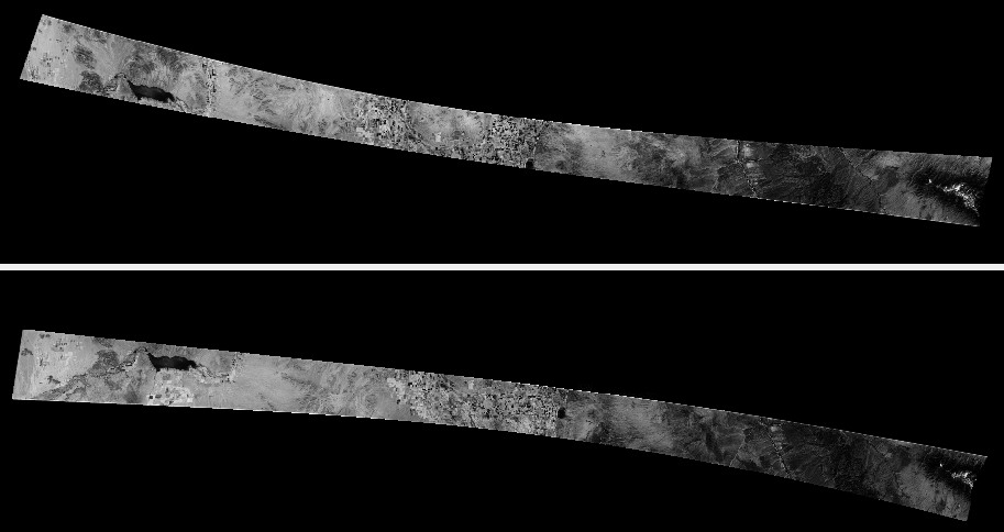
Fig. 8.40 An example of Fwd and Aft mapprojected images. Notable warping is observed.

8.28.7. Optimization of cameras

We will follow the bundle adjustment approach outlined in Section 12.2.1.3.

The quantities to be optimized are the extrinsics (camera position and starting orientation), and the intrinsics, which include the image center (optical offset), focal length, motion compensation factor, velocity vector, and the ending orientation. The last three fall under the other_intrinsics category in bundle adjustment. The command can be as follows:

bundle_adjust                               \
  fwd_sub16.tif aft_sub16.tif               \
  fwd_sub16.tsai aft_sub16.tsai             \
  --mapprojected-data                       \
    'fwd_sub16.map.tif aft_sub16.map.tif'   \
  fwd_sub16.gcp aft_sub16.gcp               \
  --inline-adjustments                      \
  --solve-intrinsics                        \
  --intrinsics-to-float other_intrinsics    \
  --intrinsics-to-share none                \
  --heights-from-dem ref.tif                \
  --heights-from-dem-uncertainty 10000      \
  --ip-per-image 100000                     \
  --ip-inlier-factor 1000                   \
  --remove-outliers-params '75 3 1000 1000' \
  --num-iterations 250                      \
  -o ba/run

We passed in the GCP files produced earlier, that have information about the ground coordinates of image corners. We made use of mapprojected images for interest point matching (Section 16.70.13).

The values for --heights-from-dem-uncertainty, --ip-per-image, --ip-inlier-factor, and --remove-outliers-params are much larger than usual, because of the very large distortion seen above. Otherwise too many valid interest points may be eliminated. Later these parameters can be tightened.

Check the produced clean match files with stereo_gui (Section 16.70.9.2). It is very important to have many of them in the corners and roughly uniformly distributed across the images. One could also consider adding the --ip-per-tile and --matches-per-tile parameters (Section 16.5.7.3). These would need some tuning at each resolution to ensure the number of matches is not overly large.

The updated cameras will be saved in the output directory. These should be validated by mapprojection as before.

We did not optimize for now the focal length and optical center, as they were known more reliably than the other intrinsics. All these can be optimized together in a subsequent pass.

See Section 16.5 for more information about bundle_adjust and the various report files that are produced.

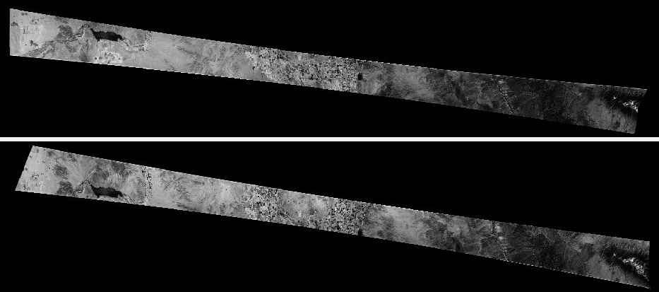
Fig. 8.41 Fwd and Aft mapprojected images, after optimization of intrinsics. The images are much better aligned.

8.28.8. Creation of a terrain model

Inspect the mapprojected images created with the new cameras. They will likely be more consistent than before. Look at the convergence angles report (Section 16.5.11.4). Hopefully this angle will have a reasonable value, such as between 10 and 40 degrees.

Run stereo and DEM creation with the mapprojected images and the asp_mgm algorithm. It is suggested to follow very closely the steps in Section 6.1.7.

8.28.9. Fixing horizontal registration errors

It is quite likely that the mapprojected images after the last bundle adjustment are much improved, but the stereo terrain model still shows systematic issues relative to the reference terrain.

Then, the dem2gcp program (Section 16.18) can be invoked to create GCP that can fix this misregistration. Pass to this program the option --max-disp if the disparity that is an input to that tool is not accurate in flat areas.

Bundle adjustment can happen with these dense GCP, while optimizing all intrinsics and extrinsics. We will share none of the intrinsics (the optical center, at least, must be unique for each individual image due to how they are scanned and cropped). Afterwards, a new stereo DEM can be created as before.

If happy enough with results at a given resolution, the cameras can be rescaled to a finer resolution and the process continued. See Section 8.26.2 for how a camera model can be modified to work at a different resolution.

8.28.10. Fixing local warping

The panoramic (OpticalBar) camera model we worked with may not have enough degrees of freedom to fix issues with local warping that arise during the storage of the film having the historical images or its subsequent digitization.

To address that, the cameras can be converted to CSM linescan format (and the images rotated by 90 degrees). See Section 16.8.1.6.

Then, the jitter solver (Section 16.39) can be employed. It is suggested to set --num-lines-per-position and --num-lines-per-orientation for this program so that there exist about 10-40 position and orientation samples along the scan direction.

This program can also accept GCP files, just like bundle_adjust. We invoked it as follows:

jitter_solve                           \
  fwd_sub16.tif aft_sub16.tif          \
  fwd_sub16.json aft_sub16.json        \
  fwd_sub16.gcp aft_sub16.gcp          \
  --match-files-prefix ba/run          \
  --num-lines-per-position 1000        \
  --num-lines-per-orientation 1000     \
  --heights-from-dem ref.tif           \
  --heights-from-dem-uncertainty 500   \
  --max-initial-reprojection-error 100 \
  --num-iterations 100                 \
  -o jitter_sub16/run

The GCP had a sigma of 100 or so, so less uncertainty than in --heights-from-dem-uncertainty, by a notable factor. At higher resolution, and if confident in GCP, one can reduce the GCP uncertainty further.

In practice we found that after one pass of the jitter solver and stereo DEM creation, it may be needed to run GCP creation with dem2gcp and bundle adjustment again to refine all the intrinsics, including focal length and lens distortion, this time with the CSM linescan model. Then, one can invoke jitter_solve one more time. Each step should offer a further improvement in results.

For fine-level control over interest point matches, dense matches from disparity are suggested (Section 12.2.4.2).

If the satellite acquired several overlapping pairs of images in quick succession, it is suggested to use them together, as that can improve the registration.

The linescan cameras are not as easy to convert to a different resolution as the OpticalBar cameras. An experimental program for this is available.