11.12. Shape-from-Shading for Earth

This example shows how to refine a terrain model for Earth using Shape-from-Shading (SfS, Section 16.67). An overview and examples for other planets are given in Section 11.1.

Fig. 11.7 Top: Four orthorectified input images showing the diversity of illumination. Bottom left: Hillshaded DEM produced with Agisoft Phtoscan. Bottom right: Hillshaded DEM refined with SfS. It can be seen that the SfS DEM has more detail. This is a small region of the test site.

Fig. 11.8 Left: Full-site hillshaded input stereo DEM (10k x 10k pixels at 0.01 m/pixel). Right: Refined full-site SfS DEM. More detail is seen. No shadow artifacts or strong dependence on albedo are observed.

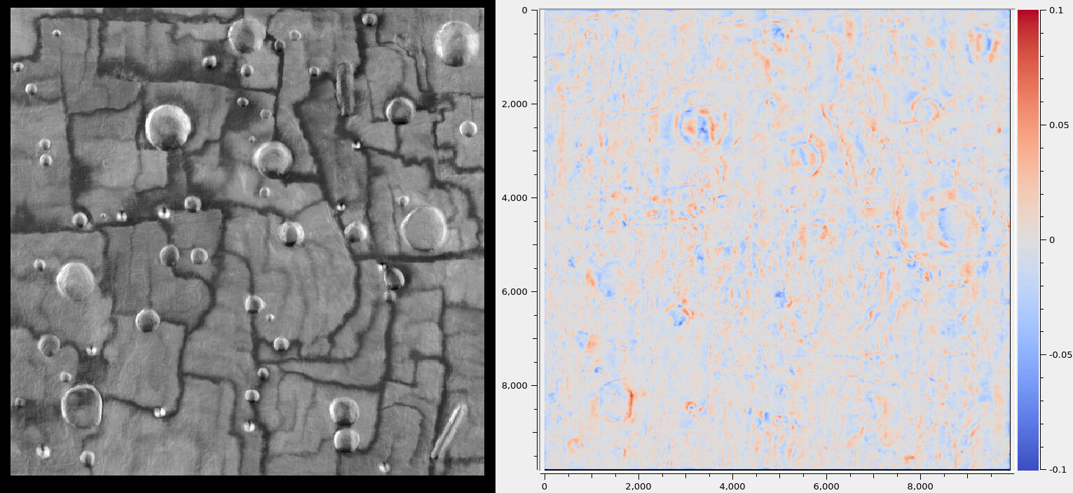
Fig. 11.9 Left: Max-lit orthoimage (this eliminates shadows). Right: SfS DEM minus the input DEM. The range of colors is between -0.1 to 0.1 meters. We do not have rigorous validation, but these results look plausible.

11.12.1. Earth-specific issues

We will produce a terrain model for the Lunar Surface Proving Ground (LSPG) at the Mojave Air and Space Port in California (35.072321 N, 118.153957 W). The site has dimensions of 100 x 100 meters.

This site is meant to mimic the topography and optical properties of Moon’s surface. It has very strong albedo variations that need modeling. Being on Earth, the site has an atmosphere that scatters sunlight, that needs to be taken into account as well.

It is likely that other rocky Earth terrains will have similar properties. Surfaces with vegetation, fresh snow, or urban areas will be very different, and likely for those the SfS method will not work well.

11.12.2. Input data

The site was imaged with an UAS flying at an elevation of about 100 meters. The images are acquired with a color frame camera, looking nadir, with dimensions of 9248 x 6944 pixels, JPEG-compressed. The ground resolution is 0.01 meters per pixel.

The camera was carefully calibrated, with its intrinsic parameters (focal length, optical center, lens distortion) known.

Five sets of images were recorded, at different times of day. Diverse illumination is very important for separating the albedo from ground reflectance and atmospheric effects.

Since SfS processes grayscale data, the red image band was used.

11.12.3. Registration and initial model

SfS expects a reasonably accurate DEM as input, that will be refined. The camera intrinsics, and their positions and orientations must be known very accurately relative to the DEM. The mapproject program (Section 16.42) can be invoked to verify the agreement between these data.

The usual process of producing such data with ASP is to run Structure-from-Motion (Section 9.1), including bundle adjustment (Section 16.5), followed by stereo (Section 3) for pairs of images with a good convergence angle (Section 8.1), terrain model creation (Section 16.57), and merge of the terrain models (Section 16.20).

If desired to refine the intrinsics, the bundle_adjust program can be run (Section 12.2.1.3), with the terrain produced so far as a constraint. If needed, alignment to a prior terrain can be done (Section 16.54), followed by carrying over the cameras (Section 16.54.14).

The stereo_gui program (Section 16.70) can help visualize the inputs, intermediate results, and final products.

11.12.4. Use of prior data

In this example, all this processing was done with Agisoft Photoscan, a commercial package that automates the steps mentioned above. It produced a terrain model, orthoimages, the camera intrinsics, and the camera positions and orientations.

11.12.5. Camera preparation

A pinhole camera model file (Section 20.1) was created for each image.

To ensure tight registration, a GCP file (Section 16.5.9) was made for each image with the gcp_gen program (Section 16.24). The inputs were the raw images, orthoimages, and the existing DEM. The invocation was as follows, for each image index i:

gcp_gen                          \
   --ip-detect-method 2          \
   --inlier-threshold 50         \
   --ip-per-tile 1000            \
   --gcp-sigma 0.1               \
   --camera-image image${i}.tif  \
   --ortho-image ortho_image.tif \
   --dem dem.tif                 \
   --output-prefix gcp/run       \
   -o gcp/image${i}.gcp

A single orthoimage was provided for all images with the same illumination.

This program’s page has more information for how to inspect and validate the GCP file.

If the camera positions and orientations are not known, such a GCP file can create the camera files from scratch (Section 9.5.2).

The images and cameras were then bundle-adjusted (Section 16.5), together with these GCP. The provided DEM was used as a constraint, with the options --heights-from-dem dem.tif --heights-from-dem-uncertainty 10.0. The latter parameter’s value was to give less weight to the DEM than to the GCP (see --gcp-sigma above), as the GCP are known to be quite accurate.

The mapproject program (Section 16.42) was run to verify that the produced cameras result in orthoimages that agree well with the input DEM and each other.

It is strongly suggested to first run this process with a small subset of the images, for example, one for each illumination. One should also inspect the various bundle_adjust report files (Section 16.5.11).

11.12.6. Terrain model preparation

The input terrain was regridded to a resolution of 0.01 meters per pixel with gdalwarp (Section 16.25):

gdalwarp         \
  -overwrite     \
  -r cubicspline \
  -tr 0.01 0.01  \
  dem.tif dem_tr0.01.tif

It is important to use a local projection in meters, such as UTM. This program can also resample an input DEM that has a geographic projection (longitude-latitude) to a local projection, with the option -t_srs.

The produced DEM was smoothed a bit, to reduce the numerical noise:

dem_mosaic            \
  --dem-blur-sigma 1  \
  dem_tr0.01.tif      \
  -o dem_tr0.01_smooth.tif

The resulting DEM can be hillshaded and visualized in stereo_gui (Section 16.70.4).

11.12.7. Illumination angles

The illumination information was specified in a file named sfs_sun_list.txt, with each line having the image name and the Sun azimuth and elevation (altitude) in degrees, in double precision, with a space as separator. The azimuth is measured clockwise from the North, and the elevation is measured from the horizon.

The SunCalc site was very useful in determining this information, given the coordinates of the site and the image acquisition time as stored in the EXIF data. One has to be mindful of local vs UTC time.

It was sufficient to use the same Sun azimuth and elevation for all images acquired in quick succession.

11.12.8. Input images

The number of input images can be very large, which can slow down the SfS program. It is suggested to divide them into groups, by illumination conditions, and ignore those outside the area of interest. ASP has logic that can help with that (Section 11.10.5).

Out of all images from a given group, a subset should be selected that covers the site fully. That can be done by mapprojecting the images onto the DEM, and then running the image_subset program (Section 16.36):

image_subset                           \
  --t_projwin min_x min_y max_x max_y  \
  --threshold 0.01                     \
  --image-list image_list.txt          \
  -o subset.txt

The values passed in via --t_projwin have the desired region extent (it can be found with gdalinfo, Section 16.25), or with stereo_gui. It is optional.

For an initial run, it is simpler to manually pick an image from each group.

The raw camera images corresponding to the union of all such subsets were put in a file named sfs_image_list.txt. The corresponding camera model files were listed in the file sfs_camera_list.txt, one per line. These must be in the same order.

11.12.9. Running SfS

The best SfS results were produced by first estimating the image exposures, haze, and a low-resolution albedo for the full site, then refining all these further per tile.

This all done under the hood by parallel_sfs (Section 16.51) in the latest build (Section 2.1). The command is:

parallel_sfs                            \
  -i dem.tif                            \
  --image-list sfs_image_list.txt       \
  --camera-list sfs_camera_list.txt     \
  --sun-angles sfs_sun_list.txt         \
  --processes 6                         \
  --threads 8                           \
  --tile-size 200                       \
  --padding 50                          \
  --blending-dist 10                    \
  --smoothness-weight 3                 \
  --robust-threshold 10                 \
  --reflectance-type 0                  \
  --num-haze-coeffs 1                   \
  --initial-dem-constraint-weight 0.001 \
  --albedo-robust-threshold 0.025       \
  --crop-input-images                   \
  --save-sparingly                      \
  --max-iterations 5                    \
  -o sfs/run

This program can be very sensitive to the smoothness weight. A higher value will produce blurred results, while a lower value will result in a noisy output. One could try various values for it that differ by a factor of 10 before refining it further.

The --robust-threshold parameter is very important for eliminating the effect of shadows. Its value should be a fraction of the difference in intensity between lit and shadowed pixels. Some experimentation may be needed to find the right value. A large value will result in visible shadow artifacts. A smaller value may require more iterations and may blur more the output.

It is strongly suggested to first run SfS on a small clip to get an intuition for the parameters (then can use the sfs program directly).

We used the Lambertian reflectance model (--reflectance-type 0). For the Moon, usually the Lunar-Lambertian model is preferred (value 1).

The produced DEM will be named sfs/run-DEM-final.tif. Other outputs are listed in Section 16.67.5.

The results are shown in Fig. 11.7.