8.16. JunoCam

JunoCam is an optical camera on the Juno spacecraft. It has been taking images of Jupiter and its satellites since 2016.

This example shows how to produce terrain models and ortho images from JunoCam images for Ganymede, the largest moon of Jupiter. These will be registered to the Voyager-Galileo global mosaic of Ganymede.

8.16.1. Fetching the data

Set (in bash):

url=https://planetarydata.jpl.nasa.gov/img/data/juno/JNOJNC_0018/DATA/RDR/JUPITER/ORBIT_34/

Download the .IMG and .LBL files for two observations:

for f in JNCR_2021158_34C00001_V01 JNCR_2021158_34C00002_V01; do
  for ext in .IMG .LBL; do
    wget $url/$f$ext
  done
done

8.16.2. Preparing the data

Ensure ISIS is installed (Section 2.3.1).

Create ISIS .cub files:

for f in JNCR_2021158_34C00001_V01 JNCR_2021158_34C00002_V01; do
    junocam2isis fr = $f.LBL to = $f.cub fullccd = yes
done

This will result in many files, because JunoCam acquires multiple overlapping images in quick succession.

Run spiceinit to get the camera pointing and other information:

for f in *.cub; do
  spiceinit from = $f web = true
done

If the web = true option does not work, the ISIS data for the juno mission needs to be downloaded, per the ISIS documentation.

We will put all these files into an img subdirectory.

Fig. 8.30 JunoCam images JNCR_2021158_34C00001_V01_0012 and JNCR_2021158_34C00002_V01_0010 as shown by stereo_gui (Section 16.70). The shared area and a couple of matching craters are highlighted.

A JunoCam image is made of 3 framelets, each about 128 pixels tall. The image width is 1648 pixels. Consecutive images have overlapping areas, which helps eliminate the effect of the gaps between the framelets.

8.16.3. External reference

We will pixel-level register the JunoCam images to the 1 km / pixel Ganymede Voyager - Galileo global mosaic.

Crop from it a portion that covers our area of interest as:

win="5745386 2069139 7893530 36002"
gdal_translate -projwin $win                        \
  Ganymede_Voyager_GalileoSSI_global_mosaic_1km.tif \
  galileo_ortho.tif

This will be stored in a subdirectory named ref.

8.16.4. Initial DEM

Both image registration and stereo DEM creation benefit from mapprojecting the JunoCam images onto a prior low-resolution DEM. A reasonably good such DEM can be created by considering the surface zero height corresponding to the earlier orthoimage clip.

Given that the elevations on Ganymede are on the order of 1 km, which is about the image resolution, this works well enough. Such a DEM is produced with image_calc (Section 16.34) as:

image_calc -c "var_0 * 0"     \
  --output-nodata-value -1e+6 \
  -d float32                  \
  ref/galileo_ortho.tif       \
  -o ref/flat_dem.tif

8.16.5. Image selection

We chose to focus on the highest resolution JunoCam images of Ganymede, as that resulted in the best terrain model. The quality of the terrain model degraded towards the limb, as expected. We worked with the images:

JNCR_2021158_34C00001_V01_0009
JNCR_2021158_34C00001_V01_0010
JNCR_2021158_34C00001_V01_0011
JNCR_2021158_34C00001_V01_0012
JNCR_2021158_34C00001_V01_0013

and corresponding images that have 34C00002 in their name.

8.16.6. Mapprojection

Each image was mapprojected (Section 16.42) at 1 km / pixel resolution, with a command such as:

mapproject --tr 1000                     \
  ref/flat_dem.tif                       \
  img/JNCR_2021158_34C00001_V01_0010.cub \
  map/JNCR_2021158_34C00001_V01_0010.map.tif

8.16.7. GCP creation

We will create GCP that ties each JunoCam image to the reference Voyager-Galileo image mosaic with gcp_gen (Section 16.24), invoked as follows:

f=JNCR_2021158_34C00001_V01_0010

gcp_gen                               \
  --ip-detect-method 0                \
  --inlier-threshold 50               \
  --ip-per-image 20000                \
  --individually-normalize            \
  --camera-image img/${f}.cub         \
  --mapproj-image map/${f}.map.tif    \
  --ortho-image ref/galileo_ortho.tif \
  --dem ref/flat_dem.tif              \
  --gcp-sigma 1000                    \
  --output-prefix gcp/run             \
  --output-gcp gcp/${f}.gcp

We set --gcp-sigma 1000, which is rather high, as we do not know the exact DEM that was employed to produce the reference image mosaic. The option --individually-normalize was essential, as these images come from different sources.

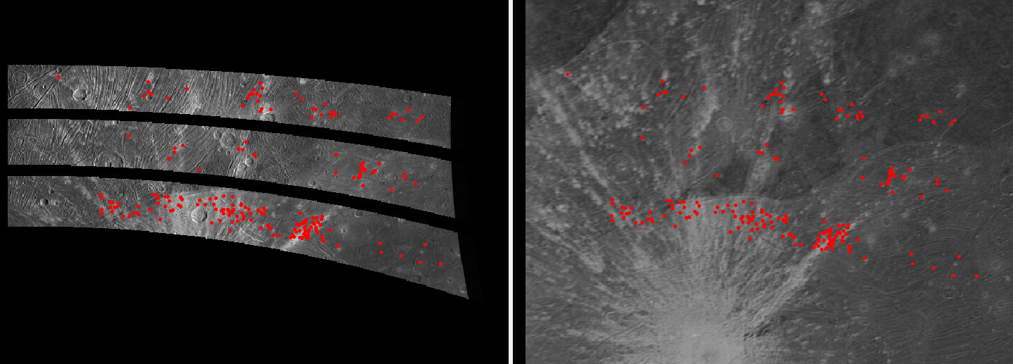
Fig. 8.31 Interest point matches between mapprojected image JNCR_2021158_34C00001_V01_0010 and the Voyager-Galileo mosaic. GCP are made from these matches.

8.16.8. Bundle adjustment

Bundle adjustment (Section 16.50) was run with the 10 images selected earlier and the GCP files:

parallel_bundle_adjust                           \
  img/JNCR_2021158_34C0000[1-2]_V01_000[9-9].cub \
  img/JNCR_2021158_34C0000[1-2]_V01_001[0-3].cub \
  --ip-per-image 20000                           \
  --num-iterations 500                           \
  gcp/*.gcp                                      \
  -o ba/run

8.16.9. Stereo terrain creation

We ran parallel_stereo on each pair of images having 34C00001 vs 34C00002 in their names. Most of these overlap and result in a DEM:

l=JNCR_2021158_34C00001_V01_0010
r=JNCR_2021158_34C00002_V01_0010
pref=stereo_map/${l}_${r}/run

parallel_stereo                      \
  map/$l.map.tif map/$r.map.tif      \
  img/$l.cub img/$r.cub              \
  --bundle-adjust-prefix ba/run      \
  --ip-per-image 20000               \
  --stereo-algorithm asp_mgm         \
  --subpixel-mode 9                  \
  --subpixel-kernel 7 7              \
  --nodata-value 0                   \
  --num-matches-from-disparity 10000 \
  ${pref}                            \
  ref/flat_dem.tif

Here we used a small subpixel-kernel of 7 x 7 pixels, to ensure as little as possible is eroded from the already narrow images. Note that the asp_mgm algorithm default corr-kernel value is 5 x 5 pixels (Section 17).

The stereo convergence angle (Section 8.1) was about 35 degrees, which is very good.

Set the output projection (the same as in the reference image mosaic):

proj='+proj=eqc +lat_ts=0 +lat_0=0 +lon_0=180 +x_0=0 +y_0=0 +R=2632344.9707 +units=m +no_defs'

Then, point2dem (Section 16.57) was run:

point2dem         \
  --t_srs "$proj" \
  --tr 1000       \
  ${pref}-PC.tif  \
  --orthoimage    \
  ${pref}-L.tif

This was followed by mosaicking of DEMs and orthoimages with dem_mosaic (Section 16.20), and colorization with colormap (Section 16.14).

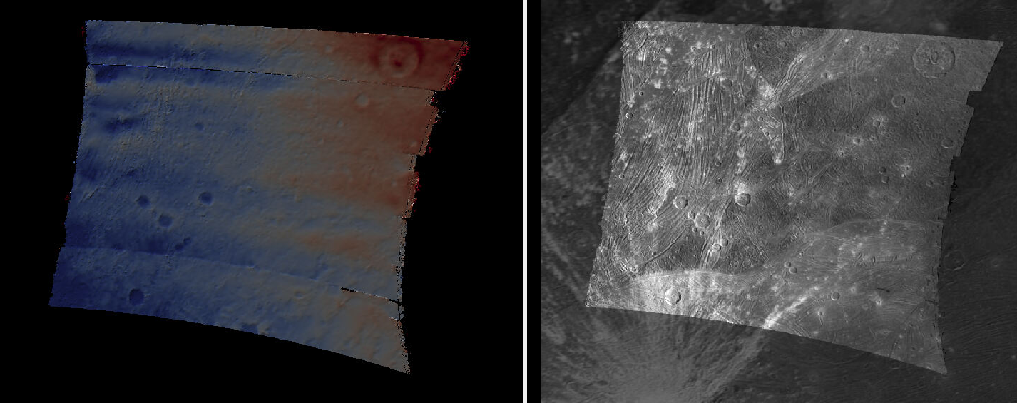
Fig. 8.32 Left: Mosaicked DEM created from stereo of JunCam images. The color range corresponds to elevations between -1500 and 1500 meters. Right: produced JunoCam orthoimage overlaid on top of the Voyager-Galileo global mosaic.

The results of this processing are shown in the figure above. Three things are notable:

• The image registration is pixel-level.

• There are some seams at the top and bottom. Those can be eliminated with more images.

• There are systematic artifacts in the elevations.

The latter issue is likely due to not well-modeled distortion and TDI effects, given the JunoCam camera design. This will be fixed in the next section.

8.16.10. Intrinsics refinement

Fig. 8.33 Left: The earlier mosaicked DEM created from stereo of JunCam images. Right: the produced DEM after optimizing the lens distortion with a DEM constraint. These are plotted with the same range of of elevations (-1500 to 1500 meters). The systematic artifacts are much less pronounced.

To address the systematic elevation artifacts, we will refine the intrinsics and extrinsics of the cameras, while using the zero elevation DEM as a ground constraint (with an uncertainty).

The approach in Section 12.2.3 is followed.

We will make use of dense matches from disparity, as in Section 12.2.4.2. The option for that, --num-matches-from-disparity, was already set in the stereo runs above. We got good results with sparse matches too, as produced by bundle_adjust, if there are a lot of them, but dense matches offer more control over the coverage.

These matches will augment existing sparse matches in the ba directory. For that, first the sparse matches will be copied to a new directory, called dense_matches. Then, we will copy on top the small number of dense matches from each stereo directory above, while removing the string -disp from each such file name, and ensuring each corresponding sparse match file is overwritten.

It is necessary to create CSM cameras (Section 8.12) for the JunoCam images, to be able to optimize the intrinsics. For the first camera, that is done with the cam_gen program (Section 16.8), with a command such as:

cam_gen img/JNCR_2021158_34C00001_V01_0010.cub          \
  --input-camera img/JNCR_2021158_34C00001_V01_0010.cub \
  --reference-dem ref/flat_dem.tif                      \
  --focal-length 1480.5905405405405405                  \
  --optical-center 814.21 600.0                         \
  --pixel-pitch 1                                       \
  --refine-camera                                       \
  --refine-intrinsics distortion                        \
  -o csm/JNCR_2021158_34C00001_V01_0010.json

The values for the focal length (in pixels) and optical center (in pixels) were obtained by peeking in the .cub file metadata.

The resulting lens distortion model is not the one for JunoCam, which has two distortion parameters, but rather the OpenCV radial-tangential model with five parameters (Section 20.3). To use the JunoCam lens distortion model, adjust the value of --distortion-type in cam_gen above.

The cam_test program (Section 16.9) can help validate that the camera is converted well.

The intrinsics of this camera are transferred without further optimization to the other cameras as:

sample=csm/JNCR_2021158_34C00001_V01_0010.json
for f in                                         \
  img/JNCR_2021158_34C0000[1-2]_V01_0009.cub     \
  img/JNCR_2021158_34C0000[1-2]_V01_001[0-3].cub \
  ; do
  g=${f/.cub/.json}
  g=csm/$(basename $g)
  cam_gen $f                                     \
    --input-camera $f                            \
    --sample-file $sample                        \
    --reference-dem ref/flat_dem.tif             \
    --pixel-pitch 1                              \
    --refine-camera                              \
    --refine-intrinsics none                     \
    -o $g
done

Next, bundle adjustment is run, with the previously optimized adjustments that reflect the registration to the reference Voyager-Galileo mosaic:

bundle_adjust                                     \
  img/JNCR_2021158_34C0000[1-2]_V01_0009.cub      \
  img/JNCR_2021158_34C0000[1-2]_V01_001[0-3].cub  \
  csm/JNCR_2021158_34C0000[1-2]_V01_0009.json     \
  csm/JNCR_2021158_34C0000[1-2]_V01_001[0-3].json \
  --input-adjustments-prefix ba/run               \
  --match-files-prefix dense_matches/run          \
  --num-iterations 50                             \
  --solve-intrinsics                              \
  --intrinsics-to-float all                       \
  --intrinsics-to-share all                       \
  --heights-from-dem ref/flat_dem.tif             \
  --heights-from-dem-uncertainty 5000             \
  gcp/*.gcp                                       \
  -o ba_rfne/run

Lastly, stereo is run with the optimized model state camera files (Section 8.12.6) saved in ba_rfne.

The result is in Fig. 8.33.

It was found that better DEMs are produced by re-mapprojecting with latest cameras and re-running stereo from scratch, rather than reusing stereo runs with the option --prev-run-prefix (Section 16.52). Likely that is because the cameras change in non-small ways.

With ISIS 9.0.0 and later, a CSM file produced as above can be embedded in the .cub file to be used with ISIS (Section 8.12.7).